Lemma First homology of a short chain complex over a PID [LNMK]
Let
be a chain complexDefinitionChain complex of free finite rank -modules over a principal ideal domain . Then
where are the invariant factors of and where .
Example Real projective plane [local-0]
Take and the real projective plane as a -complexDefinitionDelta complex: two vertices , three edges , and two triangles .
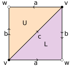
Order the vertices of each triangle so that in both, in , and in . Then
In the bases and , the Smith normal form of is
so the invariant factors are and . For , we have and , so has rank
Hence, . Now applied the theorem
Core concepts in Simplicial Homology [GYD9]
Definition Boundary and interior of [23BZ]
The boundary of is
The interior of is .
Definition Delta complex [WBTD]
A -complex is a topological space with a family of maps
for each such that ( is the standard -simplex)
- Each interior restriction of map is injective
- Each point lies in the image of interior restriction of for exactly one
- Each -boundary restriction of is equal to some where we identify the -boundary with a by the unique linear homeomorphism that preserves the order of the vertices
- A subspace is open if and only if is open for all
Definition -simplex of a -complex [K5BK]
We refer to a map as an -simplex of the -complexDefinitionDelta complex .
Definition Skeleta [8CBL]
A -complex comes with a filtration by skeleta where the -skeleton is the union of all images of simplices of dimension at most .
Example Skeleta of [local-0]
Take the -complex structure on the torus with one vertex , three edges and two triangles . Slide to see the -skeleton, and drag the torus to rotate it.
Definition Dimension of a -complex [5MJV]
A -complex is called -dimensional if and ; and it is called infinite dimensional if there is no such .
Definition Finite type and finite -complex [2A0Q]
We say that is of finite type if for each , it has only finitely many -simplices. We say is finite if it has only finitely many simplices altogether.
Definition -th simplicial chain module and -chains [Q5M5]
Let be a -complexDefinitionDelta complex. The -th simplicial chain module is the free -module with basis
Accordingly, each element of the -th simplicial chain module is a formal -linear combination
with finitely many nonzero coefficients. We call them simplicial -chains in .
Definition Boundary homomorphism (also known as differential) [EFJB]
The boundary homomorphism Definition-th simplicial chain module and -chains for is defined on the basis by
i.e. Alternatively add each restriction . Recall the third condition of -complexDefinitionDelta complex.
Lemma We have [URFG]
The composition DefinitionBoundary homomorphism (also known as differential) is the zero map.
Definition -th homology [7XRX]
The -th homology group of a chain complexDefinitionChain complex is the -module
Definition -th simplicial homology [DDAF]
The -th simplicial homology group of a -complex is the -module
Definition Chain complex [O7WN]
An algebraic chain complex is a sequence of -modules over a commutative ring
indexed over and connected by homomorphisms satisfying the condition Every -boundary is an -cycle.
關於漫畫epub [YSRC]
- 按照epub規格,只需要寫
page-progression-direction="rtl",但實際上大部分閱讀軟體需要設定pre-paginated才能把書設定成RTL - 漫畫書商產出的頁面通常是每頁一個xhtml裡面一個
img,然後直接設定(長寬是圖片像素長寬),避免圖片被裁切 - epub不可以設定成reflowable,否則有些閱讀器會讓圖片變成可點選(點了會放大圖片,然後就會無法翻頁)
MacOS網路雜記 [YUFB]
執行
ipconfig set en0 DHCP
MacOS header那邊內建的wifi UI就會壞掉(一直顯示一個驚嘆號在中間),可見這個UI的開發者應該沒有考慮到外部程式也會動到網路設定的部分xd
ifconfig awdl0 up/down
可以開關AirDrop,如果是遠端遊戲的話關掉會改善很多
Non-linear spine [A17O]
在Pattern Unification的概念中,有一類等式依賴non-linear spine,會沒有general solution,例如
這裡至少有兩組答案:
跟
Proxmox與Intel I-219v [RKU5]
前幾天遇到proxmox cluster每幾個小時就斷線,但重插網路線就會恢復,最後查到是網卡的問題https://tech.gillyb.net/proxmox-losing-network-with-intel-i-219v/。可以觀察dmesg有無
e1000e: Detected Hardware Unit Hang
確認。最後用
ethtool -K eno1 tso off gso off
關閉tso與gso之後,到目前都沒有遇到問題了xd
Theorem Computably (recursively) inseparable sets [FW2E]
Consider the following two subsets of the natural numbers:
There is no Turing machine which terminates on all inputs and separates from .
Proof [local-0]
Suppose we are given a Turing machine terminates with result or on all inputs, such that when and when . Consider the algorithm that returns a Turing machine for a given natural number: is the machine that terminates with result on every input.
Because terminates on all inputs, so does . By construction for each input : Consider the case that , then . because
but then . The same argument applies to .
By the second recursion theoremhttps://www.math.ucla.edu/~ynm/lectures/2009csl.pdf, there exists a Turing machine realizing applied to its own Gödel number, that is, . Because is or , both constant, is constant as well, say with value . Hence
so either both and lie in , or both lie in . In either case . However, for all .
資料庫其實很快 [tr-QE7I]
之前的tr在分析檔案之後把每個地址的metadata放到 _tmp/<addr>.metadata.json 裡面,而且使用 for/async,實際用我的部落格測量發現需要80.x ms,找文件查證發現其實寫入port對Racket future來說是不安全的(future-unsafe operation)https://docs.racket-lang.org/guide/parallelism.html,所以Racket其實什麼也沒做
反而還要付出runtime overhead,for線性寫完全部檔案也不過50.x ms
我最近突然想到何不放進SQLitehttps://www.sqlite.org/裡面,然後就發現
一次transaction把全部metadata寫入,只需要4.7ms!
不過這部分對全體建構時間改善就沒什麼意義了,畢竟這部分不是熱路徑,我改用SQLite也只是想減輕維護負擔
基於檔案內容判斷是否進行建置的必要性 [tr-1XYR]
tr最早的實現是
- 把使用者放在
content目錄裡面的.scrbl檔案夾進一個適當的上下文裡面,然後輸出到_tmp目錄 - 建構階段幫每一個地址開啟一個racket subprocess輸出HTML
這個實現的缺點就是慢到不行,而且如果用racket的 for/async(平行執行)常常會超出系統開啟行程的限制然後炸掉,用 for 線性執行則是需要好幾分鐘才能建構好網站,但相應的這個方法必定會進行修改
改善效能的過程中發現這個用行程調用的過程不是必須的,racket提供的 dynamic-rerequire 正好可以做到這件事,以我的網站來說建構時間降到分鐘以下的等級
接下來就是改正快取正確性,之前的快取我也是單純比較mtime(這個錯誤每個建構系統都會犯至少一次xd)。現在的版本是查看檔案原始內容,建立hash然後把一些元資料放到 _tmp/cache/<hash> 裡面
快取這裏還有一些坑,要注意把外部依賴放到變更監控裡面,所以除了一開始就遇到的 @include,我後來又加上 @tr/depends 讓使用者自己宣告一些隱藏的檔案依賴(會影響到目前卡片的建置的外部檔案變更)
但從這邊開始監控檔案的連續建置就開始出問題了,有時候修改會沒有觸發新的建構。最後用property-based test才慢慢調查到問題正在於 dynamic-rerequire,最後發現誒怎麼 dynamic-rerequire 也是比較mtimehttps://github.com/racket/racket/blob/2b83c3f3480b94c63a0c5e252b42cc1245b12c7f/racket/collects/racket/rerequire.rkt#L177來判斷要不要觸發重新載入。所以為了確保 dynamic-rerequire 在tr判斷內容有變化的時候一定會執行,我選擇把hash也放到生成的暫時檔名中。這樣內容變化就蘊含檔名變化,新的檔案就一定會觸發建構
更仔細考慮的話,目前的機制都缺乏對退出訊號的處理,所以可能遇到任意時機的中斷,不過這就留待未來處理了
用CSS計算nesting [tr-01YZ]
這是最近對tr的小修正:在渲染HTML的時候就計算並鎖死前綴數字會出問題,因為一張卡片可以被不同卡片含入(transclusion),這導致渲染結果對其他卡片來說都不正確
所以正確的解決之道是利用CSS Counters動態計算
模擬選舉演算法 [C6J7]
延續選舉演算法提到的規則,模擬一直運作下去的集群:leader定期送出心跳,一旦有節點逾時沒收到leader心跳(也可能是因為根本還沒有leader)就會轉為candidate發起選舉。讀者可以慢慢觀察leader、candidate、follower之間的轉換
你可以自己觸發故障:點一下節點可以讓它離線、上線;點一下節點之間的線可以讓那條線路故障、恢復。可以自由組合,包括同時弄掉好幾個節點看cluster在什麼情況下選不出leader。想暫停看某個瞬間可以按Pause
Colimit作為Coend [S2W7]
Coend是functor 上的一種construction,回憶一下Profunctor我們知道這種functor對左邊逆變、對右邊共變,因此對任意 有
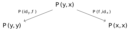
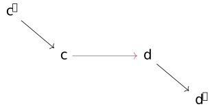
如果考慮對所有co-wedge 有一個universal construction,換句話說以下交換圖成立
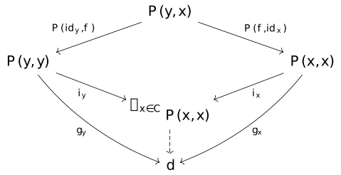
這個universal construction被稱為coend。給定functor 我們能定義一個profunctor
現在假設profunctor 有universal construction,然後我們把 按照定義機械替換成
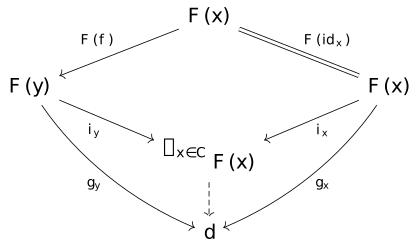
就可以看到如果 有colimit這樣的universal construction,必定與 重疊,所以colimit可以用coend表示
視Profunctor為Hom functor的generalization [2323]
Profunctor的概念是一種跨越不同範疇的Hom functor的擴充,我們先看基本定義
Definition Profunctor [local-0]
A profunctor is a functor of the form
這時候我們可以看到,重點在對於一個product category be functorial,這表示我們可以把 視為一個擬似morphism!這句話的意思是對於 跟 ,我們可以視每個 的元素為一個連接 跟 的morphism,只是它跨越不同範疇
為什麼呢?因為對一個product category be functorial就是對兩個組成範疇be functorial,表示對於 我們有
對於 我們有
這完全滿足了Hom functor的需求,因此事實上我們可以更正式的說以下構造是一個範疇:
- 取 與 的objects為objects
- 取 與 的morphisms與所有 的元素為morphisms
這又稱為a collage (or cograph) of two categories and
Tool JetKVM [55O9]
總之就是個遠端控制電腦的產品
Log Replication [6PAS]
基於選舉演算法取得leader之後,每次client發起的command應該要被leader複製到followers上
leader會向所有節點發起新增log的請求,收到過半節點ack才會回覆client這個修改成功
Raft特別要求如果有新的command但節點沒有跟上,就會拒絕並要求leader把舊的logs都複製給它,然後才會同意新的command,這表示所有節點的過半數節點有最新的logs狀態時集群才能服務client
選舉演算法 [5X6Y]
這裡簡要紀錄選舉演算法的想法
節點角色 [local-0]
節點的角色應該是以下三種之一
- Follower
- Candidate
- Leader
我們希望leader至多只有一個,只有有leader的集群才會對外提供服務
任期 [local-1]
任期可以叫term或是generation clock,用來這是第幾輪的決策,每個節點都要有這個資訊
日誌 [local-2]
日誌的每個entry應該包含
- 索引(index),每次新增entry都應該嚴格遞增的數字
- 任期(term),entry寫入時的任期
- 指令(command),要進行什麼操作
狀態轉換 [local-5]
節點啟動時可以不知道leader是誰,我們可以設定為
- term為1
- 角色為follower
- 設定定時任務檢查leader發送的heartbeat訊號
如果定時任務歸零時沒有收到leader發送的heartbeat訊號,就發起選舉;反之,重設定時任務
發起選舉 [local-3]
發起選舉可以定義為
- 把節點的term加一
- 轉換為candidate
- 投給自己
- 要求其他節點投給自己
- 等待有限時間N
現在會有幾種可能
- 在N時間內有過半節點投給自己。這時候表示自己就是leader,轉換狀態並設定循環任務不斷發送heartbeat訊號給所有節點
- 在N時間後沒有得到過半節點的票,逾時再次發起選舉(回到最前面)
- 在N時間內收到leader廣播的heartbeat,而且這個leader的term比自己大。這時候就轉變為follower,更新term並紀錄誰是leader
- 在N時間內收到其他candidate要求投給它的投票訊息,而且該投票訊息的term比自己大。這時候也轉為follower,更新term
由於candidate把term加一了才繼續,舊的領導者(比如斷線之後再連回來)的heartbeat就不會影響candidate跟其他節點
處理投票請求 [local-4]
收到投票請求的時候需要按照以下順序決策,以下的同意就表示同時要轉換為follower狀態
- candidate的term小於當前節點的term:回覆拒絕
- candidate的term大於當前節點的term:回覆同意
- candidate的term跟當前節點一樣時要繼續攤開
- 已經投過票了:請求candidate就是已經投過的candidate,回覆同意;反之回覆拒絕
- candidate的log index大於自己:回覆同意
- 其餘情況都回覆拒絕
之所以要看log index,是要避免狀態比較落後的節點成為leader,以免資料遺失
原則上就是
- 任期高者不投給任期低者
- log index高者不投給log index低者
- 每個任期只投一張票(否則過半就沒有意義)
leader如果直接看到比自己大的term(無論是heartbeat還是投票訊息),都應該放棄leader身份轉換為follower
現在我們來看逾時後投票的效果
架一個自用的Rama叢集 [rama-cluster]
Rama是Red Planet Labs創造的分散式程式平台,用Java跟Clojure寫成。這裡紀錄我把1.9.0的release解開、啟動rama cluster的過程。release zip檔案解壓出來的內容
.
├── lib
├── LICENSE.txt
├── log4j2.properties
├── logs
├── rama
├── rama.jar
├── rama.yaml
└── README.md
常駐行程 [local-0]
Rama叢集由三個常駐行程組成:
- Zookeeper:存叢集metadata。Rama透過一層叫Metastore的抽象使用它,記錄哪個節點該跑哪些module worker、以及replication的leader election
- Conductor:CLI的接口,同時提供web版的Cluster UI,負責管理模組部署
- Supervisor:每台工作機跑一個,負責處理實際執行運算的worker process的調度
各自要獨立執行:
# 內建的單機 ZK,官方標注不適合正式環境
nohup ./rama devZookeeper >/dev/null 2>&1 &
nohup ./rama conductor >/dev/null 2>&1 &
nohup ./rama supervisor >/dev/null 2>&1 &
listening ports
2000   zookeeper
1973   conductor        <- CLI client 只需要這個
8888   cluster UI
3000   supervisor HTTP  ┐
3001   worker           ├ supervisor.port.range 的前幾個 port
3002   worker           ┘
Conductor的UI開在8888,裡面有相當豐富的runtime telemetry。要讓那些數字有東西可看,要先部署內建的monitoring模組,也順手設定一下遙測的保留期避免把磁碟吃光:
./rama deploy --action launch --systemModule monitoring --tasks 4 --threads 2 --workers 1
./rama monitoringConfig --setRetention 60,90000
Problem port range的寬度限制 [local-1]
Supervisor會拿 supervisor.port.range 的第一個 port 開自己的HTTP server,worker則往後依序取用。如果預設的 [3000, 4000] 跟機器上其他東西撞到,就需要更改這個設定
我改成 [3100, 4000],結果每一個CLI指令都開始噴 Invalid config,連唯讀的 confValue 都不能用了,表示config驗證發生在所有指令的共同路徑上
文件說明只有說「port allocation range,預設 3000, 4000」,沒講到限制。試出來的結果是這樣:
[3000, 4000]   OK
[3100, 4100]   OK
[4000, 5000]   OK
[3100, 3200]   INVALID
[3001, 4000]   INVALID
所以range的寬度可能是必須恰好等於 1000,起點沒有限制。所以正確的閃避方式是平移整段ports
supervisor.port.range: [3100, 4100]
Problem Java version [local-2]
文件寫的支援範圍是Java 8/11/17/21,我機器上是 26。實測下來所有功能都正常,唯一的問題是RocksDB的JNI會噴warning
WARNING: java.lang.System::loadLibrary has been called by org.rocksdb.RocksDB
WARNING: Restricted methods will be blocked in a future release
現在只是警告,但未來的 JDK 會直接封鎖
Zookeeper 是必要的嗎? [local-3]
是的,對真正的cluster來說沒有免ZK的模式
- 只是要開發、測試 module:用
InProcessCluster,把 Rama 當成 Maven 依賴拉進專案,InProcessCluster.create()會在 process 內模擬一整個叢集,API 跟真叢集完全相同。不需要 ZK、不需要 CLI、不需要任何 daemon。官方建議的開發流程就是用 IPC 開發測試,再用 CLI 部署到真叢集 - 自用的小叢集:ZK 要有,但不需要是額外的機器。內建的
devZookeeper就是一個單機 ZK,跟 Conductor 擠同一台就好。它沒有 HA,ZK 掛了叢集就失去協調能力,自用場景通常還可以接受;不然就是要自己開一個獨立的 Apache ZooKeeper
所以ZK是必要的元件,但不一定需要額外的機器
從別台機器部署 [local-4]
這是我最想確認的使用方式:把叢集跑在別的機器上,然後從筆電下部署指令
client 端的 rama.yaml 只需要一行。我把設定刪到只剩 conductor.host,conductorReady、moduleStatus、deploy --action update 都還是能用
再來我讓 zookeeper.servers 指向一個不存在的host,上面的指令包含deploy在內照樣成功。也就是說CLI client完全不需要管Zookeeper,它只跟Conductor對話,module的jar是上傳給Conductor、再由Conductor散佈出去的
兩個要注意的地方:rama.yaml 這個檔案本身必須存在而且非空,空檔案會得到錯誤訊息 Could not find rama.yaml on classpath;另外client端的release版本必須跟叢集完全一致
所以一組最小的遠端配置是這樣。叢集那台,Conductor、Supervisor、ZK 都在上面執行:
conductor.host:
  internal: "localhost"
  external: "10.0.0.1"     # cluster 對外的 IP
local.dir: "/var/rama"
zookeeper.servers: ["localhost"]
worker.child.opts: "-Xmx4096m"
Client的設定只需要
conductor.host: "10.0.0.1"
License [local-5]
內建的免費license上限是2 台 Supervisor 節點,Conductor跟Zookeeper不計。用 rama licenseInfo 可以看到 num-nodes: 2,有效期到2117年
所以自用的天花板就是兩台工作機。再往上要跟 RPL 買 license,拿到以後用 rama upsertLicense --licensePath xxx.edn 裝上去
常用指令 [local-6]
# 部署自己的 module
rama deploy \
  --action launch \
  --jar target/app.jar \
  --module com.foo.MyModule \
  --tasks 64 \
  --threads 16 \
  --workers 8 \
  --replicationFactor 2

# 程式改動之後重新部署
rama deploy --action update \
  --jar target/app.jar \
  --module com.foo.MyModule

rama scaleExecutors --module com.foo.MyModule --threads 90 --workers 30
rama moduleStatus com.foo.MyModule
rama destroy --module com.foo.MyModule

rama repl --module com.foo.MyModule
rama runClj my.ns /path/to.jar
rama backup / supportBundle
rama shutdownCluster
--tasks 必須是 2 的次方,而且要滿足 tasks >= threads >= workers。這個約束在 deploy 跟 scaleExecutors 都適用
Video The Unreasonable Effectiveness of Constructive Data Modeling [Z4CE]
類型系統的用途是義務擴散機
什麼是CPS? [IAVH]
CPS是continuation passing style的縮寫,是一種編寫程式的風格,要理解這個概念,我們可以從為什麽要傳遞continuation開始。在循序式的語言(包含指令語言)裡面,continuation是明明白白寫出來的
- 要嘛是下一行
- 要嘛是jump到第 行
但有一種情況沒有寫,就是procedure。procedure從continuation的角度來看,是個一進一出的結構。在很多指令語言裡面都有calling convention,就是針對procedure的最佳化,因為這要求一進的時候復用現在的stack,輸入會放在特定的位置,一出的時候要把輸出寫到特定的registers
那可以多進多出嗎?可以,但我們先暫時轉向沒有明顯continuation的案例,並且討論函數式語言這種特例
在函數式語言裡面,允許傳遞lambda(匿名函數)以及其他各種高階運算式作為值,這其實給後端帶來了很大的複雜性,比如
let x := if a 1 2
in x
請問 if a 1 2 的continuation是什麼呢?是
let x := ♢ in x
♢ 用來表示任意運算式那我們是不是可以把這寫成lambda?
\♢. let x := ♢ in x
這是合法的函數式寫法嗎?是。那我們可不可以說
let x := if a 1 2
in x
等於
let k := \♢. let x := ♢ in x
in if a (k 1) (k 2)
答案還是可以。我們把這種把未來要執行的程式顯式提取出來的寫法,稱之為CPS
call/cc也就是這麼實現的。問題是,這樣傳遞的continuation通通都是同色的。比如你用call/cc做了個檔案資源清理,但呼叫的SQL連線程式丟了個exception(也用call/cc實現),這個檔案就不會被清掉了!這是資源洩漏,是非常嚴重的問題,所以scheme發展出 dynamic-wind 這個函數,用來保證裡面的運算不管發生什麼continuation跳轉都還是會執行
而且我們發現,傳統的continuation實作往往決定了一個任意的界線,例如頂層宣告以外的續延都不會被捕捉;而且我們又需要解決同色問題,所以我們發展了一些技術來處理這些
- delimited continuation:與其捕捉「所有剩下的計算(並設立任意的界線)」,不如先用prompt標出捕捉界線,abort會被prompt擋住
- 而不同用途的跳轉(exception、generator、async)可以用不同的prompt tag捕捉,他們就不會互相影響
- continuation mark這個功能則是可以把資料放到continuation frame上,之後用
current-marks沿著當下的continuation讀回來,並且保證tail call不會讓mark累積
當然,這些技術又細分成能不能多次abort,能不能多次resume等等,在runtime速度跟功能上做出取捨
最後CPS如果變成一種強制的形式,那就提供了一種優雅的編譯框架,因此這也是一種編譯理論技術。CPS變換強制把每個不明顯的control flow都打包成函數閉包,然後顯式的傳遞。做完之後有幾個性質會同時成立:每個中間值都有名字、每個呼叫都在tail position(所以call就是jump,return就是call傳進來的 k)、 化簡可以無條件使用,編譯器可以用這個IR解釋橫跨全局的控制流程,用來實現如exception等等高階控制流運算
Osiris: replicated logs [K4RQ]
Osiris是RabbitMQ使用的底層logs儲存機制,在 mix.exs 的 deps array 裡面加上
{:osiris, github: "rabbitmq/osiris", tag: "v1.13.1"}
來使用,hex.pm上面的同名專案是別的專案注意不要搞錯了。由於Osiris沒有公開API,要注意接下來講的用法未來可能被改變
準備一個資料夾給osiris,用Application env提供然後用 ensure_all_started 啟動osiris app
data_dir = ~c"/tmp/osiris"
File.mkdir_p!(data_dir)
:ok = Application.put_env(:osiris, :data_dir, data_dir)
{:ok, _apps} = Application.ensure_all_started(:osiris)
提供設定檔,單機上 leader_node 選目前的節點就可以了
config = %{
  name: "my_stream",
  epoch: 1,
  leader_node: node(),
  replica_nodes: []
}
{:ok, %{leader_pid: leader}} = :osiris.start_cluster(config)
寫入需要4個參數:osiris cluster的leader PID、writer ID、訊息序號、內容
writer_id = <<"writer-1">>
:ok = :osiris.write(leader, writer_id, 1, <<"hello">>)
:ok = :osiris.write(leader, writer_id, 2, <<"osiris">>)
成功寫入disk後會回一個 :osiris_written 訊息,所以寫入方要等這個消息傳過來,可以設定一個等待時限(這邊是5秒)
receive do
  {:osiris_written, _name, ^writer_id, seqs} ->
    IO.inspect(seqs, label: "written")
after
  5_000 -> exit(:write_timeout)
end
讀取需要建立reader,會得到一個stream state,接下來就是用 read_chunk_parsed 解析出logs的內容
{:ok, log0} = :osiris.init_reader(leader, :first, {:my_reader, []})
{entries, log1} = :osiris_log.read_chunk_parsed(log0)
IO.inspect(entries, label: "chunk 1")
讀到 :end_of_stream 之後可以關閉logs
case :osiris_log.read_chunk_parsed(log1) do
  {:end_of_stream, log2} ->
    IO.puts("end of stream")
    :osiris_log.close(log2)

  {more, log2} ->
    IO.inspect(more, label: "chunk 2")
    :osiris_log.close(log2)
end
最後關閉cluster
:ok = :osiris.stop_cluster(config)
Theorem Left/right adjoints preserve (co)/limits [0IGM]
We have
and
Proof [local-0]
Only prove right adjoints preserve limits here, left adjoints case is dual.
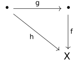
It basically invokes Hom-functors preserve limits twice
Definition J-sheaf [ZUQN]
Let be a site, a -sheaf on is a presheaf such that for each -covering sieve and for each family
such that for each and for each morphism that's -composable with
, there exists a unique element such that
for all .
Proposition For any sieve in , bigger sieve also in [7R33]
Let be a Grothendieck topology on a category . If and is a sieve on containing , then .
Proof [local-0]
The key is this: By definition of sieve, for any element , the set is a maximal sieve of ! Because let's see
because elements of are closed under composition, is the maximal sieve of :
Because all elements of also belongs to , we have ; but is the maximal sieve of , hence .
Recall that maximal sieve of belongs to , implies that for any , we have . We apply property (iii), conclude that .
Proposition Natural transformations pair of adjunctions [31KN]
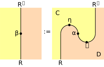
Let be two left adjoints, and their right adjoints are respectively, a natural transformation has a correspondence .
Proof [local-0]
We can construct
Definition Site [84R3]
A site is a pair consisting of a category and a Grothendieck topology on .
Definition Grothendieck topology [ZD97]
A Grothendieck topology on a category is an assignment sending any object to a collection of sieves on such that the following properties are satisfied.
Before we view the properties
- we denote with or .
- We need to define maximal sieve.
Property Maximality axiom [BEIE]
The maximal sieve .
Property Pullback stability [FXZI]
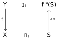
If and , then
defined by
We can represent it as
Definition Sieve [FG8Y]
A sieve on an object of a category is a family of morphisms with codomain such that closed under composition: If then for any composable we have .
We denote or .
Frames與complete Heyting algebras不同之處 [TJ21]
Theorem 3.10.2 Topology via Logic [WBA7]
Let be a lattice, then is a frame iff it is a complete Heyting algebra. See Topology via logic
Also check Theorem 3.5.2, that a frame is a complete lattice and hence has infinite meets.
可見frame就是complete Heyting algebra,那為什麼還要提供兩個名詞來稱呼他們呢?這是因為 the category of frames 跟 the category of complete Heyting algebras 裡面的morphisms不一樣!
具體來說
Definition Frame homomorphism [local-0]
A map is a frame homomorphism iff
- preserving finite meets
- preserving arbitrary joins
Definition complete Heyting algebra homomorphism [local-1]
A map is a cHa homomorphism iff
- preserving arbitrary meets
- preserving arbitrary joins
- monotone (preserving Heyting implication)
把complete lattice視為小範疇那我們就能利用範疇論的技巧 left/right adjoint functors preserves co/limits 證明他們不一樣
Proposition cHa homomorphism has left/right adjoints [local-3]
cHa homomorphism has a left adjoint and a right adjoint
Proof [local-2]
- preserves meets (limits) 所以它是right adjoint,因此有left adjoint
- preserves joins (colimits) 所以它是left adjoint,因此有right adjoint
所以相應的frame homomorphism有right adjoint但不一定有left adjoint
Idea Generate HTMLs for local cards? [tr-47YA]
tr currently produces _build/XXXX/index.html for each XXXX.scrbl in content, however, it doesn't produce HTML for local cards (write as @tr/card{...}). But _build/XXXX/ indeed has space for them, e.g. _build/XXXX/0/index.html.
Of course, this might introduce new problems
- tr-notes previously assumes there are only root-level HTMLs, would these new URIs be a problem?
- How to extract these HTMLs? e.g.
@include{...}includes pure HTML, how such forms interact with this new behaviour? - Should local cards hence be first-class citizen? e.g. Should we compute relationship between cards? Still file based? Or local address also counted in?
Regular type的導數是它的one-hole context [ag-93PB]
Details [local-0]
  {-# OPTIONS --safe --without-K #-}
  module ag-93PB where

  open import MLTT.Spartan
  open import MLTT.List
  open import UF.Equiv
  open import UF.Univalence
The Derivative of a Regular Type is its Type of One-Hole Contexts筆記
核心觀察:對一個regular type(多項式 functor)微分 得到的型別恰好就是它的「一個洞的context」,把類型視為limit與colimit構成的多項式,求導規則跟微積分一樣。這裡只用單變數functor:唯一的變數 var 表示 x
data Poly : 𝓤₀ ̇ where
  𝟘ᵖ  : Poly
  𝟙ᵖ  : Poly
  var : Poly
  _⊕_ : Poly → Poly → Poly
  _⊗_ : Poly → Poly → Poly

infixr 40 _⊕_
infixr 50 _⊗_
Definition Poly的解釋 [local-1]
polynomial解釋成型別時
  ⟦_⟧ : Poly → 𝓤₀ ̇ → 𝓤₀ ̇
  ⟦ 𝟘ᵖ    ⟧ X = 𝟘
  ⟦ 𝟙ᵖ    ⟧ X = 𝟙
  ⟦ var   ⟧ X = X
  ⟦ p ⊕ q ⟧ X = ⟦ p ⟧ X + ⟦ q ⟧ X
  ⟦ p ⊗ q ⟧ X = ⟦ p ⟧ X × ⟦ q ⟧ X
Definition 對型別微分 [local-2]
Figure 4 的前六行但排除
  ∂ : Poly → Poly
  ∂ 𝟘ᵖ      = 𝟘ᵖ
  ∂ 𝟙ᵖ      = 𝟘ᵖ
  ∂ var     = 𝟙ᵖ
  ∂ (p ⊕ q) = ∂ p ⊕ ∂ q
  ∂ (p ⊗ q) = (∂ p ⊗ q) ⊕ (p ⊗ ∂ q)
Example [local-3]
我們先看案例
  B : Poly
  B = 𝟙ᵖ ⊕ (var ⊗ var)

  _ : ∂ B = 𝟘ᵖ ⊕ ((𝟙ᵖ ⊗ var) ⊕ (var ⊗ 𝟙ᵖ))
  _ = refl

  ∂B-≃ : {X : 𝓤₀ ̇ } → ⟦ ∂ B ⟧ X ≃ (X + X)
  ∂B-≃ = qinveq to (from , from-to , to-from)
    where
    to : {X : 𝓤₀ ̇ } → ⟦ ∂ B ⟧ X → X + X
    to (inl ())
    to (inr (inl (⋆ , x))) = inl x
    to (inr (inr (x , ⋆))) = inr x

    from : {X : 𝓤₀ ̇ } → X + X → ⟦ ∂ B ⟧ X
    from (inl x) = inr (inl (⋆ , x))
    from (inr x) = inr (inr (x , ⋆))

    from-to : {X : 𝓤₀ ̇ } → (c : ⟦ ∂ B ⟧ X) → from (to c) = c
    from-to (inl ())
    from-to (inr (inl (⋆ , x))) = refl
    from-to (inr (inr (x , ⋆))) = refl

    to-from : {X : 𝓤₀ ̇ } → (v : X + X) → to (from v) = v
    to-from (inl x) = refl
    to-from (inr x) = refl

  ∂B-= : is-univalent 𝓤₀ → (X : 𝓤₀ ̇ ) → ⟦ ∂ B ⟧ X = (X + X)
  ∂B-= ua X = eqtoid ua _ _ ∂B-≃
Definition Plugging in [local-4]
給一個 one-hole context Γ : ⟦ ∂ p ⟧ X 跟一個元素 x : X,把 x 塞進洞裡重建出完整的 ⟦ p ⟧ X。
  _⋖_ : (p : Poly) {X : 𝓤₀ ̇ } → ⟦ ∂ p ⟧ X → X → ⟦ p ⟧ X
  _⋖_ 𝟘ᵖ ()
  _⋖_ 𝟙ᵖ ()
  (var ⋖ ⋆)                x = x
  ((p ⊕ q) ⋖ inl Γ)        x = inl ((p ⋖ Γ) x)
  ((p ⊕ q) ⋖ inr Γ)        x = inr ((q ⋖ Γ) x)
  ((p ⊗ q) ⋖ inl (Γ , qv)) x = (p ⋖ Γ) x , qv
  ((p ⊗ q) ⋖ inr (pv , Γ)) x = pv , (q ⋖ Γ) x
  infixl 30 _⋖_
Types on Scott's graph model [A3Q8]
基本上概念大致上就是在universal domain 中,我們可以用PERs定義出一系列classes,而這些classes的表現就如同我們想要的types,而且可以表示dependent types跟System F那種polymorphic types
表示 的類型是 ,定義成 (因為型別是PER)
這裡只聊到型別部分,關於graph model本身的運作、拓樸,可以參考Scott的論文Data Types as Lattices
PER: 正確處理 exponentiation [ag-KA1U]
From Denotational Semantics, looking backward - looking forward
Partial Equivalences as Types: First attempts的編碼有個缺點:exponentiation A => B 是定在函數 𝓟 ℕ → 𝓟 ℕ 上的關係,而不是一個 𝓟 ℕ 的關係,所以無法表示 A => B => A。這就是缺點的根源:A => B 不再是一個 Rel,因此 A => B => A 不合乎其型別的定義。
關鍵是 pairing : ℕ × ℕ ≃ ℕ,有了配對,一個 F : 𝓟 ℕ 就能被看成 ℕ 上的關係,用 application 把函數放回 𝓟 ℕ。這樣 _=>_ 就封閉成 Rel → Rel → Rel,缺點消失,A => B => A 也跟著是 PER
Details [local-0]
  {-# OPTIONS --safe --without-K #-}
  open import MLTT.Spartan
  open import MLTT.List using (List; []; _∷_; member; in-head; in-tail)
  open import UF.Base using (ap₂)
  open import UF.Equiv
  open import UF.FunExt
  open import UF.Powerset
  open import UF.Subsingletons
  open import UF.SubtypeClassifier
  open import UF.PropTrunc
  open import Naturals.Binary using (pairing)
  open import Naturals.Properties using (succ-lc; positive-not-zero)

  module ag-KA1U
    (pt : propositional-truncations-exist)
    (fe : Fun-Ext)
    (pe : propext 𝓤₀)
    where

  open PropositionalTruncation pt
  open import ag-U75Z using (_[_]_; is-PER)
我們需要讓「函數」也住在 𝓟 ℕ 裡,這樣 _=>_ 才會是封閉的 Rel → Rel → Rel
關鍵是 pairing : ℕ × ℕ ≃ ℕ,取它的正向映射 ⌜ pairing ⌝ 把一對碼壓成一個碼。因為它是equivalence,所以是injective
encode : ℕ × ℕ → ℕ
encode = ⌜ pairing ⌝

encode-lc : {a b : ℕ × ℕ} → encode a = encode b → a = b
encode-lc = equivs-are-lc encode (⌜⌝-is-equiv pairing)
graph model的application不是輸入單一個編碼餵,而是餵一個**有限的編碼集合**。我們用 List ℕ 表示有限集合,用 encode 把它壓成一個 ℕ
codeList : List ℕ → ℕ
codeList []       = 0
codeList (x ∷ xs) = succ (encode (x , codeList xs))

codeList-lc : (l l′ : List ℕ) → codeList l = codeList l′ → l = l′
codeList-lc []       []        e = refl
codeList-lc []       (y ∷ ys)  e = 𝟘-elim (positive-not-zero _ (e ⁻¹))
codeList-lc (x ∷ xs) []        e = 𝟘-elim (positive-not-zero _ e)
codeList-lc (x ∷ xs) (y ∷ ys)  e = ap₂ _∷_ (ap pr₁ q) (codeList-lc xs ys (ap pr₂ q))
  where
  q : (x , codeList xs) = (y , codeList ys)
  q = encode-lc (succ-lc e)
「有限集合 l 被 X 包含」:l 裡每個編碼都在 X 裡
_⊆ₗ_ : List ℕ → 𝓟 ℕ → 𝓤₀ ̇
l ⊆ₗ X = (k : ℕ) → member k l → k ∈ X
定義graph model的application:F ⊙ X 收集所有 m,使得存在一個有限近似 l ⊆ X,而 F 把 l(壓成的碼)送到 m
_⊙_ : 𝓟 ℕ → 𝓟 ℕ → 𝓟 ℕ
(F ⊙ X) m = (∃ l ꞉ List ℕ , (encode (codeList l , m) ∈ F) × (l ⊆ₗ X)) , ∃-is-prop
infixl 60 _⊙_
於是現在改用 F : 𝓟 ℕ → 𝓟 ℕ 的編碼版本 𝓟 ℕ,再靠 _⊙_ 取回作用。沿用記號與定義,並根據新的 Rel 定義我們需要的helpers
PER-symm : {A : Rel} → (is-PER A) → symmetric A
PER-symm per-A = per-A .pr₁
PER-trans : {A : Rel} → (is-PER A) → transitive A
PER-trans per-A = per-A .pr₂
Definition Exponentiation [local-2]
現在重新定義exponentiation
  _=>_ : Rel → Rel → Rel
  (A => B) F G = (X Y : 𝓟 ℕ) → X [ A ] Y → (F ⊙ X) [ B ] (G ⊙ Y)
  infixr 50 _=>_
把 F X 換成 F ⊙ X 後PER的證明基本上一樣
A=>B-is-PER-if-A-B-are-PERs : {A B : Rel}
     → is-PER A
     → is-PER B
     → is-PER (A => B)
A=>B-is-PER-if-A-B-are-PERs {A}{B} per-A per-B = I , II
  where
  I : symmetric (A => B)
  I F G F[A=>B]G X Y X[A]Y = goal
    where
    Y[A]X : Y [ A ] X
    Y[A]X = PER-symm per-A X Y X[A]Y

    apply : (F ⊙ Y) [ B ] (G ⊙ X)
    apply = F[A=>B]G Y X Y[A]X

    goal : (G ⊙ X) [ B ] (F ⊙ Y)
    goal = PER-symm per-B (F ⊙ Y) (G ⊙ X) apply
  II : transitive (A => B)
  II F G H F[A=>B]G G[A=>B]H X Y X[A]Y = goal
    where
    apply₁ : (F ⊙ X) [ B ] (G ⊙ Y)
    apply₁ = F[A=>B]G X Y X[A]Y

    Y[A]X : Y [ A ] X
    Y[A]X = PER-symm per-A X Y X[A]Y

    Y[A]Y : Y [ A ] Y
    Y[A]Y = PER-trans per-A Y X Y Y[A]X X[A]Y

    apply₂ : (G ⊙ Y) [ B ] (H ⊙ Y)
    apply₂ = G[A=>B]H Y Y Y[A]Y

    goal : F ⊙ X [ B ] H ⊙ Y
    goal = PER-trans per-B (F ⊙ X) (G ⊙ Y) (H ⊙ Y) apply₁ apply₂
因為封閉,套疊兩次得到 A => B => A 也是PER
A=>B=>A-is-PER : {A B : Rel}
     → is-PER A
     → is-PER B
     → is-PER (A => B => A)
A=>B=>A-is-PER per-A per-B =
  A=>B-is-PER-if-A-B-are-PERs per-A (A=>B-is-PER-if-A-B-are-PERs per-B per-A)
_=>_ 的型別現在是 Rel → Rel → Rel,缺點消失。但還有一個問題:A => B => A 既然關聯的是 𝓟 ℕ,那 fst : 𝓟 ℕ → 𝓟 ℕ → 𝓟 ℕ 活在host裡面是無法使用的,也必須被編碼成一個 𝓟 ℕ,這裡我們稱之為 K
box : ℕ → ℕ
box p = encode (codeList [] , p)

K : 𝓟 ℕ
K k = (∃ p ꞉ ℕ , k = encode (codeList (p ∷ []) , box p)) , ∃-is-prop
核心引理:K ⊙ X 再作用任何 U 的結果是 X
K-const : (X U : 𝓟 ℕ) → ((K ⊙ X) ⊙ U) = X
K-const X U = subset-extensionality pe fe to-X from-X
  where
  to-X : ((K ⊙ X) ⊙ U) ⊆ X
  to-X r = ∥∥-rec (∈-is-prop X r) I
    where
    I : (Σ l ꞉ List ℕ , (encode (codeList l , r) ∈ (K ⊙ X)) × (l ⊆ₗ U)) → r ∈ X
    I (l , kx , _) = ∥∥-rec (∈-is-prop X r) II kx
      where
      II : (Σ l₂ ꞉ List ℕ , (encode (codeList l₂ , encode (codeList l , r)) ∈ K) × (l₂ ⊆ₗ X)) → r ∈ X
      II (l₂ , ∈K , l₂⊆X) = ∥∥-rec (∈-is-prop X r) III ∈K
        where
        III : (Σ p ꞉ ℕ , encode (codeList l₂ , encode (codeList l , r)) = encode (codeList (p ∷ []) , box p)) → r ∈ X
        III (p , eq) = transport (_∈ X) (ap pr₂ inner ⁻¹) p∈X
          where
          outer : (codeList l₂ , encode (codeList l , r)) = (codeList (p ∷ []) , box p)
          outer = encode-lc eq

          inner : (codeList l , r) = (codeList [] , p)
          inner = encode-lc (ap pr₂ outer)

          l₂=p∷[] : l₂ = (p ∷ [])
          l₂=p∷[] = codeList-lc l₂ (p ∷ []) (ap pr₁ outer)

          p∈X : p ∈ X
          p∈X = l₂⊆X p (transport (member p) (l₂=p∷[] ⁻¹) in-head)

  from-X : X ⊆ ((K ⊙ X) ⊙ U)
  from-X r r∈X = ∣ [] , kx-mem , (λ k ()) ∣
    where
    kx-mem : encode (codeList [] , r) ∈ (K ⊙ X)
    kx-mem = ∣ (r ∷ []) , ∣ r , refl ∣ , sing-sub ∣
      where
      sing-sub : (r ∷ []) ⊆ₗ X
      sing-sub k in-head      = r∈X
      sing-sub k (in-tail ())
於是最後一個問題可以寫成
main : {A B : Rel} → K [ A => B => A ] K
main {A}{B} X Y X[A]Y U V U[B]V =
  transport (λ b → ((K ⊙ X) ⊙ U) [ A ] b) (K-const Y V ⁻¹)
    (transport (λ a → a [ A ] Y) (K-const X U ⁻¹) X[A]Y)
PER as types: product [ag-NN5N]
Details [local-0]
  {-# OPTIONS --safe --without-K #-}
  open import MLTT.Spartan
  open import UF.Powerset
  open import UF.PropTrunc
  open import UF.FunExt
  open import UF.Subsingletons

  module ag-NN5N
    (pt : propositional-truncations-exist)
    (fe : Fun-Ext)
    (pe : propext 𝓤₀)
    where

  open import ag-U75Z using (_[_]_; is-PER)
  open import ag-KA1U pt fe pe using (Rel; encode; PER-symm; PER-trans)
首先我們需要針對程式的projection 1跟projection 2
Fst Snd : 𝓟 ℕ → 𝓟 ℕ
Fst X n = X (encode (0 , n))
Snd X n = X (encode (1 , n))
Definition Product [local-1]
我們把product定義成
- 程式的第一部分有類型 :
Fst X [ A ] Fst Y - 且程式的第二部分有類型 :
Snd X [ B ] Snd Y
時,X [ A ×ᵣ B ] Y
  _×ᵣ_ : Rel → Rel → Rel
  (A ×ᵣ B) X Y = (Fst X [ A ] Fst Y) × (Snd X [ B ] Snd Y)
  infixr 55 _×ᵣ_
Product of PER依然是PER [local-2]
證明 A ×ᵣ B 依然是一個PER,不難看出證明就是per component而已
  A×B-is-PER : {A B : Rel}
       → is-PER A
       → is-PER B
       → is-PER (A ×ᵣ B)
  A×B-is-PER {A}{B} per-A per-B = I , II
    where
    I : symmetric (A ×ᵣ B)
    I X Y (XA , XB) =
      PER-symm per-A (Fst X) (Fst Y) XA ,
      PER-symm per-B (Snd X) (Snd Y) XB
    II : transitive (A ×ᵣ B)
    II X Y Z (XA , XB) (YA , YB) =
      PER-trans per-A (Fst X) (Fst Y) (Fst Z) XA YA ,
      PER-trans per-B (Snd X) (Snd Y) (Snd Z) XB YB
PER as types: sum [ag-MM24]
Details [local-0]
  {-# OPTIONS --safe --without-K #-}
  open import MLTT.Spartan
  open import UF.Powerset
  open import UF.PropTrunc
  open import UF.FunExt
  open import UF.Subsingletons
  open import UF.DiscreteAndSeparated using (ℕ-is-set)
  open import Naturals.Properties using (positive-not-zero)

  module ag-MM24
    (pt : propositional-truncations-exist)
    (fe : Fun-Ext)
    (pe : propext 𝓤₀)
    where

  open import ag-U75Z using (_[_]_; is-PER)
  open import ag-KA1U pt fe pe using (Rel; PER-symm; PER-trans)
  open import ag-NN5N pt fe pe using (Fst; Snd)
tag 取成 singleton:{ m } 就是只含 m 的集合
{_} : ℕ → 𝓟 ℕ
{ m } n = (m = n) , ℕ-is-set
X = ({0} , X0) 可以表示成 Fst X = { 0 } 且 Snd X = X0,inr同理
is-inl is-inr : 𝓟 ℕ → 𝓤₁ ̇
is-inl X = Fst X = { 0 }
is-inr X = Fst X = { 1 }
輔助引理證明不可能既是inl又是inr
inl-and-inr-is-impossible : (X : 𝓟 ℕ) → is-inl X → is-inr X → 𝟘
inl-and-inr-is-impossible X p q =
  positive-not-zero 0 (transport (0 ∈_) (p ⁻¹ ∙ q) refl)
Definition Sum [local-1]
我們把sum定義成
- 要嘛兩邊都是inl、且
Snd X [ A ] Snd Y - 不然就是兩邊都是inr、且
Snd X [ B ] Snd Y
  _+ᵣ_ : Rel → Rel → Rel
  (A +ᵣ B) X Y = (is-inl X × is-inl Y × (Snd X [ A ] Snd Y))
               + (is-inr X × is-inr Y × (Snd X [ B ] Snd Y))
  infixr 54 _+ᵣ_
Sum of PER依然是PER [local-2]
A +ᵣ B 依然是PER。symmetric跟transitivity的同向情況都是per component;混合情況用 inl-and-inr-is-impossible 推出矛盾排除
  A+B-is-PER : {A B : Rel}
       → is-PER A
       → is-PER B
       → is-PER (A +ᵣ B)
  A+B-is-PER {A}{B} per-A per-B = I , II
    where
    I : symmetric (A +ᵣ B)
    I X Y (inl (lX , lY , XA)) =
      inl (lY , lX , PER-symm per-A (Snd X) (Snd Y) XA)
    I X Y (inr (rX , rY , XB)) =
      inr (rY , rX , PER-symm per-B (Snd X) (Snd Y) XB)
    II : transitive (A +ᵣ B)
    II X Y Z (inl (lX , _ , XA)) (inl (_ , lZ , YA)) =
      inl (lX , lZ , PER-trans per-A (Snd X) (Snd Y) (Snd Z) XA YA)
    II X Y Z (inr (rX , _ , XB)) (inr (_ , rZ , YB)) =
      inr (rX , rZ , PER-trans per-B (Snd X) (Snd Y) (Snd Z) XB YB)
    II X Y Z (inl (_ , lY , _)) (inr (rY , _ , _)) =
      𝟘-elim (inl-and-inr-is-impossible Y lY rY)
    II X Y Z (inr (_ , rY , _)) (inl (lY , _ , _)) =
      𝟘-elim (inl-and-inr-is-impossible Y lY rY)
PER as types: dependent product & sum [ag-BQXB]
Details [local-0]
  {-# OPTIONS --safe --without-K #-}
  open import MLTT.Spartan
  open import UF.Powerset
  open import UF.PropTrunc
  open import UF.FunExt
  open import UF.Subsingletons

  module ag-BQXB
    (pt : propositional-truncations-exist)
    (fe : Fun-Ext)
    (pe : propext 𝓤₀)
    where

  open import ag-U75Z using (_[_]_; is-PER)
  open import ag-KA1U pt fe pe using (Rel; PER-symm; PER-trans; _⊙_; _=>_)
  open import ag-NN5N pt fe pe using (Fst; Snd; _×ᵣ_)
依賴型別由一族 B : 𝓟 ℕ → Rel 給出。要讓它在 A 的商空間上良好定義,需要 B 在 A:U [ A ] V 時滿足 B U = B V
dependent sum:Fst X 由 A 分類,Snd X 由 B (Fst X) 分類
Σᵣ : (A : Rel) → (𝓟 ℕ → Rel) → Rel
Σᵣ A B X Y = (Fst X [ A ] Fst Y) × (Snd X [ B (Fst X) ] Snd Y)
infixr 55 Σᵣ
dependent product:把 F 作用在被 A 分類的 X 上,結果由 B X 分類
Πᵣ : (A : Rel) → (𝓟 ℕ → Rel) → Rel
Πᵣ A B F G = (X Y : 𝓟 ℕ) → X [ A ] Y → (F ⊙ X) [ B X ] (G ⊙ Y)
infixr 50 Πᵣ
Dependent sum of PER依然是PER [local-1]
Per component提出證明,依賴的部分要靠 B U = B V 把證明在 B (Fst X) 與 B (Fst Y) 之間搬移
  Σ-is-PER : {A : Rel} {B : 𝓟 ℕ → Rel}
       → is-PER A
       → ((U : 𝓟 ℕ) → is-PER (B U))
       → ({U V : 𝓟 ℕ} → U [ A ] V → B U = B V)
       → is-PER (Σᵣ A B)
  Σ-is-PER {A}{B} per-A per-B resp = I , II
    where
    I : symmetric (Σᵣ A B)
    I X Y (p , q) =
      PER-symm per-A (Fst X) (Fst Y) p ,
      PER-symm (per-B (Fst Y)) (Snd X) (Snd Y)
        (transport (λ R → Snd X [ R ] Snd Y) (resp p) q)
    II : transitive (Σᵣ A B)
    II X Y Z (p₁ , q₁) (p₂ , q₂) =
      PER-trans per-A (Fst X) (Fst Y) (Fst Z) p₁ p₂ ,
      PER-trans (per-B (Fst X)) (Snd X) (Snd Y) (Snd Z) q₁
        (transport (λ R → Snd Y [ R ] Snd Z) (resp p₁ ⁻¹) q₂)
Dependent product of PER依然是PER [local-2]
結構與 _=>_ 相同,只是每次套用後都要把型別 B Y 搬回 B X
  Π-is-PER : {A : Rel} {B : 𝓟 ℕ → Rel}
       → is-PER A
       → ((U : 𝓟 ℕ) → is-PER (B U))
       → ({U V : 𝓟 ℕ} → U [ A ] V → B U = B V)
       → is-PER (Πᵣ A B)
  Π-is-PER {A}{B} per-A per-B resp = I , II
    where
    I : symmetric (Πᵣ A B)
    I F G F[Π]G X Y X[A]Y = goal
      where
      Y[A]X : Y [ A ] X
      Y[A]X = PER-symm per-A X Y X[A]Y

      apply : (F ⊙ Y) [ B Y ] (G ⊙ X)
      apply = F[Π]G Y X Y[A]X

      apply' : (F ⊙ Y) [ B X ] (G ⊙ X)
      apply' = transport (λ R → (F ⊙ Y) [ R ] (G ⊙ X)) (resp Y[A]X) apply

      goal : (G ⊙ X) [ B X ] (F ⊙ Y)
      goal = PER-symm (per-B X) (F ⊙ Y) (G ⊙ X) apply'
    II : transitive (Πᵣ A B)
    II F G H F[Π]G G[Π]H X Y X[A]Y = goal
      where
      apply₁ : (F ⊙ X) [ B X ] (G ⊙ Y)
      apply₁ = F[Π]G X Y X[A]Y

      Y[A]X : Y [ A ] X
      Y[A]X = PER-symm per-A X Y X[A]Y

      Y[A]Y : Y [ A ] Y
      Y[A]Y = PER-trans per-A Y X Y Y[A]X X[A]Y

      apply₂ : (G ⊙ Y) [ B Y ] (H ⊙ Y)
      apply₂ = G[Π]H Y Y Y[A]Y

      apply₂' : (G ⊙ Y) [ B X ] (H ⊙ Y)
      apply₂' = transport (λ R → (G ⊙ Y) [ R ] (H ⊙ Y)) (resp Y[A]X) apply₂

      goal : (F ⊙ X) [ B X ] (H ⊙ Y)
      goal = PER-trans (per-B X) (F ⊙ X) (G ⊙ Y) (H ⊙ Y) apply₁ apply₂'
Polymorphic types [ag-8LAS]
Details [local-0]
  {-# OPTIONS --safe --without-K #-}
  open import MLTT.Spartan
  open import UF.Powerset
  open import UF.PropTrunc
  open import UF.FunExt
  open import UF.Subsingletons

  module ag-8LAS
    (pt : propositional-truncations-exist)
    (fe : Fun-Ext)
    (pe : propext 𝓤₀)
    where

  open import ag-U75Z using (_[_]_; is-PER)
  open import ag-KA1U pt fe pe using (Rel; PER-symm; PER-trans)
Polymorphic type量化的不是元素,而是型別(PER)本身。一支program住在 ∀X. T(X) 裡的意思是不管 X 是哪個型別,它都住在 T(X) 裡。在這裡型別就是 PER,所以這恰好是把所有instance F A 取交集
(M , N)屬於∀ᵣ Fiff對每個PERA都有M [ F A ] N
交集量化了所有 Rel,落在比 Rel 高一階的universe,但Agda的universe是predicative的,所以要提供一個新名字 Rel⁺
Rel⁺ : 𝓤₂ ⁺ ̇
Rel⁺ = 𝓟 ℕ → 𝓟 ℕ → 𝓤₂ ̇

∀ᵣ : (Rel → Rel) → Rel⁺
∀ᵣ F M N = (A : Rel) → is-PER A → M [ F A ] N
PER的交集依然是PER [local-1]
逐點證明:symmetric與transitive 都在固定的 A 上呼叫 F A 自己的PER結構,再把 A 量化回去
  ∀-is-PER : (F : Rel → Rel)
       → ((A : Rel) → is-PER A → is-PER (F A))
       → is-PER (∀ᵣ F)
  ∀-is-PER F per-F = I , II
    where
    I : symmetric (∀ᵣ F)
    I M N M[∀F]N A per-A =
      PER-symm (per-F A per-A) M N (M[∀F]N A per-A)
    II : transitive (∀ᵣ F)
    II M N L M[∀F]N N[∀F]L A per-A =
      PER-trans (per-F A per-A) M N L (M[∀F]N A per-A) (N[∀F]L A per-A)
Polymorphic types [ag-8LAS]
Details [local-0]
  {-# OPTIONS --safe --without-K #-}
  open import MLTT.Spartan
  open import UF.Powerset
  open import UF.PropTrunc
  open import UF.FunExt
  open import UF.Subsingletons

  module ag-8LAS
    (pt : propositional-truncations-exist)
    (fe : Fun-Ext)
    (pe : propext 𝓤₀)
    where

  open import ag-U75Z using (_[_]_; is-PER)
  open import ag-KA1U pt fe pe using (Rel; PER-symm; PER-trans)
Polymorphic type量化的不是元素,而是型別(PER)本身。一支program住在 ∀X. T(X) 裡的意思是不管 X 是哪個型別,它都住在 T(X) 裡。在這裡型別就是 PER,所以這恰好是把所有instance F A 取交集
(M , N)屬於∀ᵣ Fiff對每個PERA都有M [ F A ] N
交集量化了所有 Rel,落在比 Rel 高一階的universe,但Agda的universe是predicative的,所以要提供一個新名字 Rel⁺
Rel⁺ : 𝓤₂ ⁺ ̇
Rel⁺ = 𝓟 ℕ → 𝓟 ℕ → 𝓤₂ ̇

∀ᵣ : (Rel → Rel) → Rel⁺
∀ᵣ F M N = (A : Rel) → is-PER A → M [ F A ] N
PER的交集依然是PER [local-1]
逐點證明:symmetric與transitive 都在固定的 A 上呼叫 F A 自己的PER結構,再把 A 量化回去
  ∀-is-PER : (F : Rel → Rel)
       → ((A : Rel) → is-PER A → is-PER (F A))
       → is-PER (∀ᵣ F)
  ∀-is-PER F per-F = I , II
    where
    I : symmetric (∀ᵣ F)
    I M N M[∀F]N A per-A =
      PER-symm (per-F A per-A) M N (M[∀F]N A per-A)
    II : transitive (∀ᵣ F)
    II M N L M[∀F]N N[∀F]L A per-A =
      PER-trans (per-F A per-A) M N L (M[∀F]N A per-A) (N[∀F]L A per-A)
PER as types: dependent product & sum [ag-BQXB]
Details [local-0]
  {-# OPTIONS --safe --without-K #-}
  open import MLTT.Spartan
  open import UF.Powerset
  open import UF.PropTrunc
  open import UF.FunExt
  open import UF.Subsingletons

  module ag-BQXB
    (pt : propositional-truncations-exist)
    (fe : Fun-Ext)
    (pe : propext 𝓤₀)
    where

  open import ag-U75Z using (_[_]_; is-PER)
  open import ag-KA1U pt fe pe using (Rel; PER-symm; PER-trans; _⊙_; _=>_)
  open import ag-NN5N pt fe pe using (Fst; Snd; _×ᵣ_)
依賴型別由一族 B : 𝓟 ℕ → Rel 給出。要讓它在 A 的商空間上良好定義,需要 B 在 A:U [ A ] V 時滿足 B U = B V
dependent sum:Fst X 由 A 分類,Snd X 由 B (Fst X) 分類
Σᵣ : (A : Rel) → (𝓟 ℕ → Rel) → Rel
Σᵣ A B X Y = (Fst X [ A ] Fst Y) × (Snd X [ B (Fst X) ] Snd Y)
infixr 55 Σᵣ
dependent product:把 F 作用在被 A 分類的 X 上,結果由 B X 分類
Πᵣ : (A : Rel) → (𝓟 ℕ → Rel) → Rel
Πᵣ A B F G = (X Y : 𝓟 ℕ) → X [ A ] Y → (F ⊙ X) [ B X ] (G ⊙ Y)
infixr 50 Πᵣ
Dependent sum of PER依然是PER [local-1]
Per component提出證明,依賴的部分要靠 B U = B V 把證明在 B (Fst X) 與 B (Fst Y) 之間搬移
  Σ-is-PER : {A : Rel} {B : 𝓟 ℕ → Rel}
       → is-PER A
       → ((U : 𝓟 ℕ) → is-PER (B U))
       → ({U V : 𝓟 ℕ} → U [ A ] V → B U = B V)
       → is-PER (Σᵣ A B)
  Σ-is-PER {A}{B} per-A per-B resp = I , II
    where
    I : symmetric (Σᵣ A B)
    I X Y (p , q) =
      PER-symm per-A (Fst X) (Fst Y) p ,
      PER-symm (per-B (Fst Y)) (Snd X) (Snd Y)
        (transport (λ R → Snd X [ R ] Snd Y) (resp p) q)
    II : transitive (Σᵣ A B)
    II X Y Z (p₁ , q₁) (p₂ , q₂) =
      PER-trans per-A (Fst X) (Fst Y) (Fst Z) p₁ p₂ ,
      PER-trans (per-B (Fst X)) (Snd X) (Snd Y) (Snd Z) q₁
        (transport (λ R → Snd Y [ R ] Snd Z) (resp p₁ ⁻¹) q₂)
Dependent product of PER依然是PER [local-2]
結構與 _=>_ 相同,只是每次套用後都要把型別 B Y 搬回 B X
  Π-is-PER : {A : Rel} {B : 𝓟 ℕ → Rel}
       → is-PER A
       → ((U : 𝓟 ℕ) → is-PER (B U))
       → ({U V : 𝓟 ℕ} → U [ A ] V → B U = B V)
       → is-PER (Πᵣ A B)
  Π-is-PER {A}{B} per-A per-B resp = I , II
    where
    I : symmetric (Πᵣ A B)
    I F G F[Π]G X Y X[A]Y = goal
      where
      Y[A]X : Y [ A ] X
      Y[A]X = PER-symm per-A X Y X[A]Y

      apply : (F ⊙ Y) [ B Y ] (G ⊙ X)
      apply = F[Π]G Y X Y[A]X

      apply' : (F ⊙ Y) [ B X ] (G ⊙ X)
      apply' = transport (λ R → (F ⊙ Y) [ R ] (G ⊙ X)) (resp Y[A]X) apply

      goal : (G ⊙ X) [ B X ] (F ⊙ Y)
      goal = PER-symm (per-B X) (F ⊙ Y) (G ⊙ X) apply'
    II : transitive (Πᵣ A B)
    II F G H F[Π]G G[Π]H X Y X[A]Y = goal
      where
      apply₁ : (F ⊙ X) [ B X ] (G ⊙ Y)
      apply₁ = F[Π]G X Y X[A]Y

      Y[A]X : Y [ A ] X
      Y[A]X = PER-symm per-A X Y X[A]Y

      Y[A]Y : Y [ A ] Y
      Y[A]Y = PER-trans per-A Y X Y Y[A]X X[A]Y

      apply₂ : (G ⊙ Y) [ B Y ] (H ⊙ Y)
      apply₂ = G[Π]H Y Y Y[A]Y

      apply₂' : (G ⊙ Y) [ B X ] (H ⊙ Y)
      apply₂' = transport (λ R → (G ⊙ Y) [ R ] (H ⊙ Y)) (resp Y[A]X) apply₂

      goal : (F ⊙ X) [ B X ] (H ⊙ Y)
      goal = PER-trans (per-B X) (F ⊙ X) (G ⊙ Y) (H ⊙ Y) apply₁ apply₂'
PER as types: sum [ag-MM24]
Details [local-0]
  {-# OPTIONS --safe --without-K #-}
  open import MLTT.Spartan
  open import UF.Powerset
  open import UF.PropTrunc
  open import UF.FunExt
  open import UF.Subsingletons
  open import UF.DiscreteAndSeparated using (ℕ-is-set)
  open import Naturals.Properties using (positive-not-zero)

  module ag-MM24
    (pt : propositional-truncations-exist)
    (fe : Fun-Ext)
    (pe : propext 𝓤₀)
    where

  open import ag-U75Z using (_[_]_; is-PER)
  open import ag-KA1U pt fe pe using (Rel; PER-symm; PER-trans)
  open import ag-NN5N pt fe pe using (Fst; Snd)
tag 取成 singleton:{ m } 就是只含 m 的集合
{_} : ℕ → 𝓟 ℕ
{ m } n = (m = n) , ℕ-is-set
X = ({0} , X0) 可以表示成 Fst X = { 0 } 且 Snd X = X0,inr同理
is-inl is-inr : 𝓟 ℕ → 𝓤₁ ̇
is-inl X = Fst X = { 0 }
is-inr X = Fst X = { 1 }
輔助引理證明不可能既是inl又是inr
inl-and-inr-is-impossible : (X : 𝓟 ℕ) → is-inl X → is-inr X → 𝟘
inl-and-inr-is-impossible X p q =
  positive-not-zero 0 (transport (0 ∈_) (p ⁻¹ ∙ q) refl)
Definition Sum [local-1]
我們把sum定義成
- 要嘛兩邊都是inl、且
Snd X [ A ] Snd Y - 不然就是兩邊都是inr、且
Snd X [ B ] Snd Y
  _+ᵣ_ : Rel → Rel → Rel
  (A +ᵣ B) X Y = (is-inl X × is-inl Y × (Snd X [ A ] Snd Y))
               + (is-inr X × is-inr Y × (Snd X [ B ] Snd Y))
  infixr 54 _+ᵣ_
Sum of PER依然是PER [local-2]
A +ᵣ B 依然是PER。symmetric跟transitivity的同向情況都是per component;混合情況用 inl-and-inr-is-impossible 推出矛盾排除
  A+B-is-PER : {A B : Rel}
       → is-PER A
       → is-PER B
       → is-PER (A +ᵣ B)
  A+B-is-PER {A}{B} per-A per-B = I , II
    where
    I : symmetric (A +ᵣ B)
    I X Y (inl (lX , lY , XA)) =
      inl (lY , lX , PER-symm per-A (Snd X) (Snd Y) XA)
    I X Y (inr (rX , rY , XB)) =
      inr (rY , rX , PER-symm per-B (Snd X) (Snd Y) XB)
    II : transitive (A +ᵣ B)
    II X Y Z (inl (lX , _ , XA)) (inl (_ , lZ , YA)) =
      inl (lX , lZ , PER-trans per-A (Snd X) (Snd Y) (Snd Z) XA YA)
    II X Y Z (inr (rX , _ , XB)) (inr (_ , rZ , YB)) =
      inr (rX , rZ , PER-trans per-B (Snd X) (Snd Y) (Snd Z) XB YB)
    II X Y Z (inl (_ , lY , _)) (inr (rY , _ , _)) =
      𝟘-elim (inl-and-inr-is-impossible Y lY rY)
    II X Y Z (inr (_ , rY , _)) (inl (lY , _ , _)) =
      𝟘-elim (inl-and-inr-is-impossible Y lY rY)
PER as types: product [ag-NN5N]
Details [local-0]
  {-# OPTIONS --safe --without-K #-}
  open import MLTT.Spartan
  open import UF.Powerset
  open import UF.PropTrunc
  open import UF.FunExt
  open import UF.Subsingletons

  module ag-NN5N
    (pt : propositional-truncations-exist)
    (fe : Fun-Ext)
    (pe : propext 𝓤₀)
    where

  open import ag-U75Z using (_[_]_; is-PER)
  open import ag-KA1U pt fe pe using (Rel; encode; PER-symm; PER-trans)
首先我們需要針對程式的projection 1跟projection 2
Fst Snd : 𝓟 ℕ → 𝓟 ℕ
Fst X n = X (encode (0 , n))
Snd X n = X (encode (1 , n))
Definition Product [local-1]
我們把product定義成
- 程式的第一部分有類型 :
Fst X [ A ] Fst Y - 且程式的第二部分有類型 :
Snd X [ B ] Snd Y
時,X [ A ×ᵣ B ] Y
  _×ᵣ_ : Rel → Rel → Rel
  (A ×ᵣ B) X Y = (Fst X [ A ] Fst Y) × (Snd X [ B ] Snd Y)
  infixr 55 _×ᵣ_
Product of PER依然是PER [local-2]
證明 A ×ᵣ B 依然是一個PER,不難看出證明就是per component而已
  A×B-is-PER : {A B : Rel}
       → is-PER A
       → is-PER B
       → is-PER (A ×ᵣ B)
  A×B-is-PER {A}{B} per-A per-B = I , II
    where
    I : symmetric (A ×ᵣ B)
    I X Y (XA , XB) =
      PER-symm per-A (Fst X) (Fst Y) XA ,
      PER-symm per-B (Snd X) (Snd Y) XB
    II : transitive (A ×ᵣ B)
    II X Y Z (XA , XB) (YA , YB) =
      PER-trans per-A (Fst X) (Fst Y) (Fst Z) XA YA ,
      PER-trans per-B (Snd X) (Snd Y) (Snd Z) XB YB
PER: 正確處理 exponentiation [ag-KA1U]
From Denotational Semantics, looking backward - looking forward
Partial Equivalences as Types: First attempts的編碼有個缺點:exponentiation A => B 是定在函數 𝓟 ℕ → 𝓟 ℕ 上的關係,而不是一個 𝓟 ℕ 的關係,所以無法表示 A => B => A。這就是缺點的根源:A => B 不再是一個 Rel,因此 A => B => A 不合乎其型別的定義。
關鍵是 pairing : ℕ × ℕ ≃ ℕ,有了配對,一個 F : 𝓟 ℕ 就能被看成 ℕ 上的關係,用 application 把函數放回 𝓟 ℕ。這樣 _=>_ 就封閉成 Rel → Rel → Rel,缺點消失,A => B => A 也跟著是 PER
Details [local-0]
  {-# OPTIONS --safe --without-K #-}
  open import MLTT.Spartan
  open import MLTT.List using (List; []; _∷_; member; in-head; in-tail)
  open import UF.Base using (ap₂)
  open import UF.Equiv
  open import UF.FunExt
  open import UF.Powerset
  open import UF.Subsingletons
  open import UF.SubtypeClassifier
  open import UF.PropTrunc
  open import Naturals.Binary using (pairing)
  open import Naturals.Properties using (succ-lc; positive-not-zero)

  module ag-KA1U
    (pt : propositional-truncations-exist)
    (fe : Fun-Ext)
    (pe : propext 𝓤₀)
    where

  open PropositionalTruncation pt
  open import ag-U75Z using (_[_]_; is-PER)
我們需要讓「函數」也住在 𝓟 ℕ 裡,這樣 _=>_ 才會是封閉的 Rel → Rel → Rel
關鍵是 pairing : ℕ × ℕ ≃ ℕ,取它的正向映射 ⌜ pairing ⌝ 把一對碼壓成一個碼。因為它是equivalence,所以是injective
encode : ℕ × ℕ → ℕ
encode = ⌜ pairing ⌝

encode-lc : {a b : ℕ × ℕ} → encode a = encode b → a = b
encode-lc = equivs-are-lc encode (⌜⌝-is-equiv pairing)
graph model的application不是輸入單一個編碼餵,而是餵一個**有限的編碼集合**。我們用 List ℕ 表示有限集合,用 encode 把它壓成一個 ℕ
codeList : List ℕ → ℕ
codeList []       = 0
codeList (x ∷ xs) = succ (encode (x , codeList xs))

codeList-lc : (l l′ : List ℕ) → codeList l = codeList l′ → l = l′
codeList-lc []       []        e = refl
codeList-lc []       (y ∷ ys)  e = 𝟘-elim (positive-not-zero _ (e ⁻¹))
codeList-lc (x ∷ xs) []        e = 𝟘-elim (positive-not-zero _ e)
codeList-lc (x ∷ xs) (y ∷ ys)  e = ap₂ _∷_ (ap pr₁ q) (codeList-lc xs ys (ap pr₂ q))
  where
  q : (x , codeList xs) = (y , codeList ys)
  q = encode-lc (succ-lc e)
「有限集合 l 被 X 包含」:l 裡每個編碼都在 X 裡
_⊆ₗ_ : List ℕ → 𝓟 ℕ → 𝓤₀ ̇
l ⊆ₗ X = (k : ℕ) → member k l → k ∈ X
定義graph model的application:F ⊙ X 收集所有 m,使得存在一個有限近似 l ⊆ X,而 F 把 l(壓成的碼)送到 m
_⊙_ : 𝓟 ℕ → 𝓟 ℕ → 𝓟 ℕ
(F ⊙ X) m = (∃ l ꞉ List ℕ , (encode (codeList l , m) ∈ F) × (l ⊆ₗ X)) , ∃-is-prop
infixl 60 _⊙_
於是現在改用 F : 𝓟 ℕ → 𝓟 ℕ 的編碼版本 𝓟 ℕ,再靠 _⊙_ 取回作用。沿用記號與定義,並根據新的 Rel 定義我們需要的helpers
PER-symm : {A : Rel} → (is-PER A) → symmetric A
PER-symm per-A = per-A .pr₁
PER-trans : {A : Rel} → (is-PER A) → transitive A
PER-trans per-A = per-A .pr₂
Definition Exponentiation [local-2]
現在重新定義exponentiation
  _=>_ : Rel → Rel → Rel
  (A => B) F G = (X Y : 𝓟 ℕ) → X [ A ] Y → (F ⊙ X) [ B ] (G ⊙ Y)
  infixr 50 _=>_
把 F X 換成 F ⊙ X 後PER的證明基本上一樣
A=>B-is-PER-if-A-B-are-PERs : {A B : Rel}
     → is-PER A
     → is-PER B
     → is-PER (A => B)
A=>B-is-PER-if-A-B-are-PERs {A}{B} per-A per-B = I , II
  where
  I : symmetric (A => B)
  I F G F[A=>B]G X Y X[A]Y = goal
    where
    Y[A]X : Y [ A ] X
    Y[A]X = PER-symm per-A X Y X[A]Y

    apply : (F ⊙ Y) [ B ] (G ⊙ X)
    apply = F[A=>B]G Y X Y[A]X

    goal : (G ⊙ X) [ B ] (F ⊙ Y)
    goal = PER-symm per-B (F ⊙ Y) (G ⊙ X) apply
  II : transitive (A => B)
  II F G H F[A=>B]G G[A=>B]H X Y X[A]Y = goal
    where
    apply₁ : (F ⊙ X) [ B ] (G ⊙ Y)
    apply₁ = F[A=>B]G X Y X[A]Y

    Y[A]X : Y [ A ] X
    Y[A]X = PER-symm per-A X Y X[A]Y

    Y[A]Y : Y [ A ] Y
    Y[A]Y = PER-trans per-A Y X Y Y[A]X X[A]Y

    apply₂ : (G ⊙ Y) [ B ] (H ⊙ Y)
    apply₂ = G[A=>B]H Y Y Y[A]Y

    goal : F ⊙ X [ B ] H ⊙ Y
    goal = PER-trans per-B (F ⊙ X) (G ⊙ Y) (H ⊙ Y) apply₁ apply₂
因為封閉,套疊兩次得到 A => B => A 也是PER
A=>B=>A-is-PER : {A B : Rel}
     → is-PER A
     → is-PER B
     → is-PER (A => B => A)
A=>B=>A-is-PER per-A per-B =
  A=>B-is-PER-if-A-B-are-PERs per-A (A=>B-is-PER-if-A-B-are-PERs per-B per-A)
_=>_ 的型別現在是 Rel → Rel → Rel,缺點消失。但還有一個問題:A => B => A 既然關聯的是 𝓟 ℕ,那 fst : 𝓟 ℕ → 𝓟 ℕ → 𝓟 ℕ 活在host裡面是無法使用的,也必須被編碼成一個 𝓟 ℕ,這裡我們稱之為 K
box : ℕ → ℕ
box p = encode (codeList [] , p)

K : 𝓟 ℕ
K k = (∃ p ꞉ ℕ , k = encode (codeList (p ∷ []) , box p)) , ∃-is-prop
核心引理:K ⊙ X 再作用任何 U 的結果是 X
K-const : (X U : 𝓟 ℕ) → ((K ⊙ X) ⊙ U) = X
K-const X U = subset-extensionality pe fe to-X from-X
  where
  to-X : ((K ⊙ X) ⊙ U) ⊆ X
  to-X r = ∥∥-rec (∈-is-prop X r) I
    where
    I : (Σ l ꞉ List ℕ , (encode (codeList l , r) ∈ (K ⊙ X)) × (l ⊆ₗ U)) → r ∈ X
    I (l , kx , _) = ∥∥-rec (∈-is-prop X r) II kx
      where
      II : (Σ l₂ ꞉ List ℕ , (encode (codeList l₂ , encode (codeList l , r)) ∈ K) × (l₂ ⊆ₗ X)) → r ∈ X
      II (l₂ , ∈K , l₂⊆X) = ∥∥-rec (∈-is-prop X r) III ∈K
        where
        III : (Σ p ꞉ ℕ , encode (codeList l₂ , encode (codeList l , r)) = encode (codeList (p ∷ []) , box p)) → r ∈ X
        III (p , eq) = transport (_∈ X) (ap pr₂ inner ⁻¹) p∈X
          where
          outer : (codeList l₂ , encode (codeList l , r)) = (codeList (p ∷ []) , box p)
          outer = encode-lc eq

          inner : (codeList l , r) = (codeList [] , p)
          inner = encode-lc (ap pr₂ outer)

          l₂=p∷[] : l₂ = (p ∷ [])
          l₂=p∷[] = codeList-lc l₂ (p ∷ []) (ap pr₁ outer)

          p∈X : p ∈ X
          p∈X = l₂⊆X p (transport (member p) (l₂=p∷[] ⁻¹) in-head)

  from-X : X ⊆ ((K ⊙ X) ⊙ U)
  from-X r r∈X = ∣ [] , kx-mem , (λ k ()) ∣
    where
    kx-mem : encode (codeList [] , r) ∈ (K ⊙ X)
    kx-mem = ∣ (r ∷ []) , ∣ r , refl ∣ , sing-sub ∣
      where
      sing-sub : (r ∷ []) ⊆ₗ X
      sing-sub k in-head      = r∈X
      sing-sub k (in-tail ())
於是最後一個問題可以寫成
main : {A B : Rel} → K [ A => B => A ] K
main {A}{B} X Y X[A]Y U V U[B]V =
  transport (λ b → ((K ⊙ X) ⊙ U) [ A ] b) (K-const Y V ⁻¹)
    (transport (λ a → a [ A ] Y) (K-const X U ⁻¹) X[A]Y)
Partial Equivalences as Types: First attempts [ag-U75Z]
From Denotational Semantics, looking backward - looking forward
這裡嘗試用agda表示Partial Equivalences as Types
{-# OPTIONS --safe --without-K #-}
open import MLTT.Spartan
open import UF.Equiv
open import UF.Powerset
open import UF.SubtypeClassifier

module ag-U75Z where
我們用agda表示relation
Rel : 𝓤₁ ̇
Rel = 𝓟 ℕ → 𝓟 ℕ → 𝓤₀ ̇
定義一個輔助閱讀的表達記號 X [ R ] Y
_[_]_ : {X : 𝓤 ̇ } → X → (X → X → 𝓥 ̇ ) → X → 𝓥 ̇
x [ R ] y = R x y
一個relation是PER表示它是symmetric且transitive
is-PER : {X : 𝓤 ̇} → (X → X → 𝓥 ̇) → 𝓤 ⊔ 𝓥  ̇
is-PER R = symmetric R × transitive R
提取用的helpers
PER-symm : {A : Rel} → (is-PER A) → symmetric A
PER-symm per-A = per-A .pr₁
PER-trans : {A : Rel} → (is-PER A) → transitive A
PER-trans per-A = per-A .pr₂
現在可以定義PER的exponentiation
_=>_ : Rel → Rel → (𝓟 ℕ → 𝓟 ℕ) → (𝓟 ℕ → 𝓟 ℕ) → 𝓤₁ ̇
(A => B) F G = (X Y : 𝓟 ℕ) → X [ A ] Y → (F X) [ B ] (G Y)
infixr 50 _=>_
我們希望證明exponentiation依然是一個PER(當然也因此是type)
A=>B-is-PER-if-A-B-are-PERs : {A B : Rel}
     → is-PER A
     → is-PER B
     → is-PER (A => B)
A=>B-is-PER-if-A-B-are-PERs {A}{B} per-A per-B = I , II
  where
  I : symmetric (A => B)
  I F G F[A=>B]G X Y X[A]Y = goal
    where
    Y[A]X : Y [ A ] X
    Y[A]X = PER-symm per-A X Y X[A]Y

    swap : Y [ A ] X → (F Y) [ B ] (G X)
    swap = F[A=>B]G Y X

    apply : (F Y) [ B ] (G X)
    apply = swap Y[A]X

    goal : (G X) [ B ] (F Y)
    goal = PER-symm per-B (F Y) (G X) apply
  II : transitive (A => B)
  II F G H F[A=>B]G G[A=>B]H X Y X[A]Y = goal
    where
    apply₁ : (F X) [ B ] (G Y)
    apply₁ = F[A=>B]G X Y X[A]Y

    Y[A]X : Y [ A ] X
    Y[A]X = PER-symm per-A X Y X[A]Y

    Y[A]Y : Y [ A ] Y
    Y[A]Y = PER-trans per-A Y X Y Y[A]X X[A]Y

    apply₂ : (G Y) [ B ] (H Y)
    apply₂ = G[A=>B]H Y Y Y[A]Y

    goal : F X [ B ] H Y
    goal = PER-trans per-B (F X) (G Y) (H Y) apply₁ apply₂
確認這真的表示了函數類型的概念
this-is-really-function-type : {A B : Rel}
  → (F : 𝓟 ℕ → 𝓟 ℕ) → F [ A => B ] F
  → ((X : 𝓟 ℕ) → X [ A ] X → F X [ B ] F X)
this-is-really-function-type {A}{B} F F:A=>B X X:A = F:A=>B X X X:A
編碼的缺點 [local-0]
我本來覺得用 𝓟 ℕ → 𝓟 ℕ → 𝓤₀ ̇ 表示relation就好,這個編碼也成功的回答了前兩個問題。但當我們需要表示 A => B => A 時,因為 B => A 不是一個 𝓟 ℕ,所以程式就寫不出來了,比如第三個問題
fst : 𝓟 ℕ → 𝓟 ℕ → 𝓟 ℕ
fst x y = x

main : {A B : Rel} → fst [ A => B => A ] fst
Lemma HoTT 2.1.4 [violet-EVW3]
\import std/id

\universe 𝓤S 𝓤

\operator "\x ⋅ \y" => trans x y
  \associativity: \left
Unit laws [local-0]
\let trans-refl-l{A : universe 𝓤} -> {x : A} -> {y : A} -> (p : x = y) -> (refl ⋅ p) = p (i.e. {A : universe 𝓤} -> {x : A} -> {y : A} -> (p : Id x y) -> Id (trans refl p) p) {Auniverse 𝓤 : 𝓤universe S 𝓤} {xA yA : Auniverse 𝓤} (px = y (i.e. Id x y) : xA = yA) : (refl ⋅ p{A : universe 𝓤} -> {x : A} -> {y : A} -> {z : A} -> (_ : x = y) -> (_ : y = z) -> x = z (i.e. {A : universe 𝓤} -> {x : A} -> {y : A} -> {z : A} -> (_ : Id x y) -> (_ : Id y z) -> Id x z)) = px = y (i.e. Id x y) => refl
\let trans-refl-r{A : universe 𝓤} -> {x : A} -> {y : A} -> (p : x = y) -> (p ⋅ refl) = p (i.e. {A : universe 𝓤} -> {x : A} -> {y : A} -> (p : Id x y) -> Id (trans p refl) p) {Auniverse 𝓤 : 𝓤universe S 𝓤} {xA yA : Auniverse 𝓤} : (px = y (i.e. Id x y) : xA = yA) -> (px = i (i.e. Id x i) ⋅ refl) = px = i (i.e. Id x i) \where
  trans-refl-r px = y (i.e. Id x y) <= \elim p$-2 = $-3 (i.e. Id $-2 $-3)
  | trans-refl-r{A : universe 𝓤} -> {x : A} -> {y : A} -> (p : x = y) -> (p ⋅ refl) = p (i.e. {A : universe 𝓤} -> {x : A} -> {y : A} -> (p : Id x y) -> Id (trans p refl) p) refl{A : universe 𝓤} -> {x : A} -> x = x (i.e. {A : universe 𝓤} -> {x : A} -> Id x x) => refl{A : universe 𝓤} -> {x : A} -> x = x (i.e. {A : universe 𝓤} -> {x : A} -> Id x x)
Inverse laws [local-1]
\let trans-sym-l{A : universe 𝓤} -> {x : A} -> {y : A} -> (p : x = y) -> ((sym p) ⋅ p) = refl (i.e. {A : universe 𝓤} -> {x : A} -> {y : A} -> (p : Id x y) -> Id (trans (sym p) p) refl) {Auniverse 𝓤 : 𝓤universe S 𝓤} {xA yA : Auniverse 𝓤} : (px = y (i.e. Id x y) : xA = yA) -> ((sym{A : universe 𝓤} -> {x : A} -> {y : A} -> (_ : x = y) -> y = x (i.e. {A : universe 𝓤} -> {x : A} -> {y : A} -> (_ : Id x y) -> Id y x) px = i (i.e. Id x i)) ⋅ px = i (i.e. Id x i)) = refl \where
  trans-sym-l px = y (i.e. Id x y) <= \elim p$-2 = $-3 (i.e. Id $-2 $-3)
  | trans-sym-l{A : universe 𝓤} -> {x : A} -> {y : A} -> (p : x = y) -> ((sym p) ⋅ p) = refl (i.e. {A : universe 𝓤} -> {x : A} -> {y : A} -> (p : Id x y) -> Id (trans (sym p) p) refl) refl{A : universe 𝓤} -> {x : A} -> x = x (i.e. {A : universe 𝓤} -> {x : A} -> Id x x) => refl{A : universe 𝓤} -> {x : A} -> x = x (i.e. {A : universe 𝓤} -> {x : A} -> Id x x)

\let trans-sym-r{A : universe 𝓤} -> {x : A} -> {y : A} -> (p : x = y) -> (p ⋅ (sym p)) = refl (i.e. {A : universe 𝓤} -> {x : A} -> {y : A} -> (p : Id x y) -> Id (trans p (sym p)) refl) {Auniverse 𝓤 : 𝓤universe S 𝓤} {xA yA : Auniverse 𝓤} : (px = y (i.e. Id x y) : xA = yA) -> (px = i (i.e. Id x i) ⋅ (sym{A : universe 𝓤} -> {x : A} -> {y : A} -> (_ : x = y) -> y = x (i.e. {A : universe 𝓤} -> {x : A} -> {y : A} -> (_ : Id x y) -> Id y x) px = i (i.e. Id x i))) = refl \where
  trans-sym-r px = y (i.e. Id x y) <= \elim p$-2 = $-3 (i.e. Id $-2 $-3)
  | trans-sym-r{A : universe 𝓤} -> {x : A} -> {y : A} -> (p : x = y) -> (p ⋅ (sym p)) = refl (i.e. {A : universe 𝓤} -> {x : A} -> {y : A} -> (p : Id x y) -> Id (trans p (sym p)) refl) refl{A : universe 𝓤} -> {x : A} -> x = x (i.e. {A : universe 𝓤} -> {x : A} -> Id x x) => refl{A : universe 𝓤} -> {x : A} -> x = x (i.e. {A : universe 𝓤} -> {x : A} -> Id x x)
Involution [local-2]
\let sym-sym{A : universe 𝓤} -> {x : A} -> {y : A} -> (p : x = y) -> (sym (sym p)) = p (i.e. {A : universe 𝓤} -> {x : A} -> {y : A} -> (p : Id x y) -> Id (sym (sym p)) p) {Auniverse 𝓤 : 𝓤universe S 𝓤} {xA yA : Auniverse 𝓤} : (px = y (i.e. Id x y) : xA = yA) -> (sym{A : universe 𝓤} -> {x : A} -> {y : A} -> (_ : x = y) -> y = x (i.e. {A : universe 𝓤} -> {x : A} -> {y : A} -> (_ : Id x y) -> Id y x) (sym{A : universe 𝓤} -> {x : A} -> {y : A} -> (_ : x = y) -> y = x (i.e. {A : universe 𝓤} -> {x : A} -> {y : A} -> (_ : Id x y) -> Id y x) px = i (i.e. Id x i))) = px = i (i.e. Id x i) \where
  sym-sym px = y (i.e. Id x y) <= \elim p$-2 = $-3 (i.e. Id $-2 $-3)
  | sym-sym{A : universe 𝓤} -> {x : A} -> {y : A} -> (p : x = y) -> (sym (sym p)) = p (i.e. {A : universe 𝓤} -> {x : A} -> {y : A} -> (p : Id x y) -> Id (sym (sym p)) p) refl{A : universe 𝓤} -> {x : A} -> x = x (i.e. {A : universe 𝓤} -> {x : A} -> Id x x) => refl{A : universe 𝓤} -> {x : A} -> x = x (i.e. {A : universe 𝓤} -> {x : A} -> Id x x)
Associativity [local-3]
\let trans-assoc{A : universe 𝓤} -> {w : A} -> {x : A} -> {y : A} -> {z : A} -> (p : w = x) -> (q : x = y) -> (r : y = z) -> ((p ⋅ q) ⋅ r) = (p ⋅ (q ⋅ r)) (i.e. {A : universe 𝓤} -> {w : A} -> {x : A} -> {y : A} -> {z : A} -> (p : Id w x) -> (q : Id x y) -> (r : Id y z) -> Id (trans (trans p q) r) (trans p (trans q r))) {Auniverse 𝓤 : 𝓤universe S 𝓤} {wA xA yA zA : Auniverse 𝓤}
  : (pw = x (i.e. Id w x) : wA = xA) -> (qi = y (i.e. Id i y) : xA = yA) -> (ry = z (i.e. Id y z) : yA = zA)
    -> (pw = i (i.e. Id w i) ⋅ qi = y (i.e. Id i y) ⋅ ry = z (i.e. Id y z)) = (pw = i (i.e. Id w i) ⋅ (qi = y (i.e. Id i y) ⋅ ry = z (i.e. Id y z))) \where
  trans-assoc pw = x (i.e. Id w x) qx = y (i.e. Id x y) ry = z (i.e. Id y z) <= \elim p$-2 = $-3 (i.e. Id $-2 $-3)
  | trans-assoc{A : universe 𝓤} -> {w : A} -> {x : A} -> {y : A} -> {z : A} -> (p : w = x) -> (q : x = y) -> (r : y = z) -> ((p ⋅ q) ⋅ r) = (p ⋅ (q ⋅ r)) (i.e. {A : universe 𝓤} -> {w : A} -> {x : A} -> {y : A} -> {z : A} -> (p : Id w x) -> (q : Id x y) -> (r : Id y z) -> Id (trans (trans p q) r) (trans p (trans q r))) refl{A : universe 𝓤} -> {x : A} -> x = x (i.e. {A : universe 𝓤} -> {x : A} -> Id x x) q r => refl{A : universe 𝓤} -> {x : A} -> x = x (i.e. {A : universe 𝓤} -> {x : A} -> Id x x)
Tool Soufflé [souffle]
Soufflé is a variant of Datalog for tool designers crafting analyses in Horn clauses. Soufflé synthesizes a native parallel C++ program from a logic specification.
Local operator 與 Nucleus [ag-X72H]
Local operator 跟 Nucleus 有什麼關聯?
{-# OPTIONS --safe --without-K #-}
open import MLTT.Spartan
open import UF.Base
open import UF.Equiv
open import UF.FunExt
open import UF.PropTrunc
open import UF.Subsingletons
open import UF.SubtypeClassifier
open import UF.SubtypeClassifier-Properties
open import UF.Size
open import UF.Logic
open import UF.Subsingletons-FunExt
open import UF.EquivalenceExamples

module ag-X72H
  (pt : propositional-truncations-exist)
  (fe : Fun-Ext)
  (pe : propext 𝓤)
  (ρ  : propositional-resizing (𝓤 ⁺) 𝓤)
  where

open Conjunction
open Universal   fe
open Implication fe

open import ag-V2O7 pt fe pe ρ
open import ag-5W9X pt fe pe ρ
open import ag-GY8B pt fe pe ρ
open import ag-95LU pt fe pe ρ
open import ag-GK6B pt fe pe ρ
open import ag-3HBW pt fe pe ρ
open is-local-operator
Ω 𝓤 本身就是一個 frame(the initial frame
𝟎-𝔽𝕣𝕞)
Ω 𝓤- order 是
⇒ - meet 是
∧
於是 Nucleus Ωᶠ 正好可與 is-local-operator
對照
open import Locales.Frame        pt fe
open import Locales.InitialFrame pt fe
open import Locales.Sublocale.Nucleus pt fe

Ωᶠ : Frame (𝓤 ⁺) 𝓤 𝓤
Ωᶠ = 𝟎-𝔽𝕣𝕞 pe
Nucleus 的 inflationary + idempotent + meet-preserving 可以推得 local
operator 的 monotone + unit + idempotent,單調性由
nuclei-are-monotone 提供
nucleus-to-local-operator : (n : Nucleus Ωᶠ) → is-local-operator (pr₁ n)
nucleus-to-local-operator n@(j , inf , idm , _) .mono p q p⇒q =
  nuclei-are-monotone Ωᶠ n (p , q) p⇒q
nucleus-to-local-operator n@(j , inf , idm , _) .unit = inf ⊤
nucleus-to-local-operator n@(j , inf , idm , _) .idem p = idm p
local operator 可以推得 Nucleus
local-operator-to-nucleus :
  (j : Ω 𝓤 → Ω 𝓤)
  → is-local-operator j
  → Nucleus Ωᶠ
local-operator-to-nucleus j j-is-local-op =
  j , inflationary , idempotent , meet-preserving
  where
  inflationary : is-inflationary Ωᶠ j holds
  inflationary x = LO-infl j-is-local-op x

  idempotent : is-idempotent Ωᶠ j holds
  idempotent x = idem j-is-local-op x

  I : (p : Ω 𝓤) → L j p = j p
  I p = Ω-extensionality pe fe ⇒-dir ⇐-dir
    where
    ⇒-dir : (L j p ⇒ j p) holds
    ⇒-dir ljp = εL j p ljp (j p) (inflationary p , idempotent p)
    ⇐-dir : (j p ⇒ L j p) holds
    ⇐-dir jp = ηL j p II
      where
      II : (L⁺ j p) holds
      II q (p⇒q , jq⇒q) = jq⇒q (mono j-is-local-op p q p⇒q jp)

  is-meet-preserving : (Ω 𝓤 → Ω 𝓤) → 𝓤 ⁺ ̇
  is-meet-preserving j = (p q : Ω 𝓤) → j (p ∧ q) = j p ∧ j q
  meet-preserving : is-meet-preserving j
  meet-preserving p q =
    j (p ∧ q)      =⟨ (I (p ∧ q)) ⁻¹ ⟩
    L j (p ∧ q)    =⟨ L-preserves-arg-∧ (j , j-is-local-op .mono) p q ⟩
    L j p ∧ L j q  =⟨ ap₂ _∧_ (I p) (I q) ⟩
    j p ∧ j q      ∎
所以從 monotone 也可以得到 Nucleus
L-nucleus : (m : Mon) → Nucleus Ωᶠ
L-nucleus m =
  local-operator-to-nucleus (L (monotone-function m))
                            (L-is-local-operator m)
is-local-operator 也是 proposition
is-local-operator-is-prop : (j : Ω 𝓤 → Ω 𝓤) → is-prop (is-local-operator j)
is-local-operator-is-prop j = equiv-to-prop unfold Fields-is-prop
  where
  Fields : 𝓤 ⁺ ̇
  Fields =   is-monotone j holds
           × (⊤ {𝓤} ⇒ j ⊤) holds
           × ((p : Ω 𝓤) → (j (j p) ⇒ j p) holds)

  unfold : is-local-operator j ≃ Fields
  unfold = qinveq (λ r → mono r , unit r , idem r)
                  ( (λ (m , u , i) → record { mono = m ; unit = u ; idem = i })
                  , (λ _ → refl) , (λ _ → refl) )

  Fields-is-prop : is-prop Fields
  Fields-is-prop = ×-is-prop (holds-is-prop (is-monotone j))
                (×-is-prop (holds-is-prop (⊤ {𝓤} ⇒ j ⊤))
                           (Π-is-prop fe (λ p → holds-is-prop (j (j p) ⇒ j p))))
型別 Loc 與 Nucleus Ωᶠ 等價
Loc : 𝓤 ⁺ ̇
Loc = Σ j ꞉ (Ω 𝓤 → Ω 𝓤) , is-local-operator j

Loc-≃-Nucleus : Loc ≃ Nucleus Ωᶠ
Loc-≃-Nucleus = Σ-cong predicates-agree
  where
  predicates-agree : (j : Ω 𝓤 → Ω 𝓤)
    → is-local-operator j ≃ is-nucleus Ωᶠ j holds
  predicates-agree j =
    logically-equivalent-props-are-equivalent
      (is-local-operator-is-prop j)
      (holds-is-prop (is-nucleus Ωᶠ j))
      ([⇒]) ([⇐])
    where
    [⇒] : is-local-operator j → is-nucleus Ωᶠ j holds
    [⇒] j-lo =
      pr₂ (local-operator-to-nucleus j j-lo)

    [⇐] : is-nucleus Ωᶠ j holds → is-local-operator j
    [⇐] n = nucleus-to-local-operator (j , n)
Proposition 保持元素的 meet [ag-3HBW]
保持有限 meet 是運算子格上的 meet,這裡要證明的是 是否保持 frame 元素的 meet,也就是
這正是 是不是 nucleus 的關鍵條件
{-# OPTIONS --safe --without-K #-}
open import MLTT.Spartan
open import UF.FunExt
open import UF.PropTrunc
open import UF.Subsingletons
open import UF.SubtypeClassifier
open import UF.Size
open import UF.Logic

module ag-3HBW
  (pt : propositional-truncations-exist)
  (fe : Fun-Ext)
  (pe : propext 𝓤)
  (ρ  : propositional-resizing (𝓤 ⁺) 𝓤)
  where

open Conjunction
open Universal   fe
open Implication fe

open import ag-V2O7 pt fe pe ρ
open import ag-5W9X pt fe pe ρ
open import ag-GY8B pt fe pe ρ
open import ag-95LU pt fe pe ρ
open is-local-operator
⊤ ⇒ s 等於 s 成立。
⊤⇒ : (s : Ω 𝓤) → (⊤ {𝓤} ⇒ s) = s
⊤⇒ s = Ω-extensionality pe fe (λ ⊤⇒s → ⊤⇒s ⊤-holds) (λ sh _ → sh)
(⇐) 方向:L f p ∧ L f q → L f (p ∧ q)
L-preserves-arg-∧-⇐ : (f : Ω 𝓤 → Ω 𝓤) (p q : Ω 𝓤)
                    → (L f p holds × L f q holds)
                    → L f (p ∧ q) holds
L-preserves-arg-∧-⇐ f p q (L[f][p] , L[f][q]) = ηL f (p ∧ q) I
  where
  L[p] = εL f p L[f][p]
  L[q] = εL f q L[f][q]

  I : (L⁺ f (p ∧ q)) holds
  I s (p∧q⇒s , fs⇒s) = L[q] s (q⇒s , fs⇒s)
    where
    -- 在 L f p 代入 r := (q ⇒ s),取得 q ⇒ s
    q⇒s : (q ⇒ s) holds
    q⇒s = L[p] (q ⇒ s) (uncurried , f⟨q⇒s⟩⇒)
      where
      uncurried : (p ⇒ (q ⇒ s)) holds
      uncurried ph qh = p∧q⇒s (ph , qh)

      -- f (q ⇒ s) ⇒ (q ⇒ s):q 成立時 (q ⇒ s) = s,故 f (q ⇒ s) = f s
      f⟨q⇒s⟩⇒ : (f (q ⇒ s) ⇒ (q ⇒ s)) holds
      f⟨q⇒s⟩⇒ y qh = fs⇒s (transport (λ - → f - holds) ⟨q⇒s⟩=s y)
        where
        ⟨q⇒s⟩=s : (q ⇒ s) = s
        ⟨q⇒s⟩=s = ap (_⇒ s) (holds-gives-equal-⊤ pe fe q qh) ∙ ⊤⇒ s
(⇒) 方向:由 L f 的單調性(因為 L(f) 是 local operator)配上
p ∧ q ⇒ p、p ∧ q ⇒ q。
L-preserves-arg-∧-⇒ : (m : Mon) (p q : Ω 𝓤)
   → L (monotone-function m) (p ∧ q) holds
   → (L (monotone-function m) p holds × L (monotone-function m) q holds)
L-preserves-arg-∧-⇒ m p q lf[p∧q] = mn (p ∧ q) p pr₁ lf[p∧q]
                                   , mn (p ∧ q) q pr₂ lf[p∧q]
  where
  mn = L-is-local-operator m .mono
合併得到
L-preserves-arg-∧ : (m : Mon) (p q : Ω 𝓤)
   → L (monotone-function m) (p ∧ q)
   = L (monotone-function m) p ∧ L (monotone-function m) q
L-preserves-arg-∧ m p q =
  Ω-extensionality pe fe (L-preserves-arg-∧-⇒ m p q)
                         (L-preserves-arg-∧-⇐ (monotone-function m) p q)
Basic Subtoposes of the Effective Topos:Proposition 1.2 [ECDG]
Lee 與 van Oosten 閱讀筆記,Proposition 1.2
為什麼要在意 local operator?因為一個 topos 的子拓樸(subtopos)跟 上的 local operator 一一對應:子拓樸就是對有限極限封閉、且包含函子有保持有限極限左伴隨的全子範疇,而這樣的資料剛好被 上的某類自映射編碼。所以「構造並區分 local operator」等於「構造並區分子拓樸」。
舞台上的角色: 是子物件分類子, 是 的單調自映射, 則是 local operator。論文指出 與 都是 internal locale,因為 Proposition 1.2 這個 Topos Theory 的一個 folklore 結果:包含映射 有一個左伴隨 保持有限 meet
首先看用到的四個定義
Definition Mon(單調自映射) [ag-V2O7]
{-# OPTIONS --safe --without-K #-}
open import MLTT.Spartan
open import UF.FunExt
open import UF.PropTrunc
open import UF.Subsingletons
open import UF.SubtypeClassifier
open import UF.Size
open import UF.Logic

module ag-V2O7
  (pt : propositional-truncations-exist)
  (fe : Fun-Ext)
  (pe : propext 𝓤)
  (ρ  : propositional-resizing (𝓤 ⁺) 𝓤)
  where

open Conjunction
open Universal   fe
open Implication fe
Monotone map 是 Ω 的自映射 f : Ω → Ω,滿足
p ⇒ q 蘊涵 f p ⇒ f q
is-monotone : (Ω 𝓤 → Ω 𝓤) → Ω (𝓤 ⁺)
is-monotone f = Ɐ p ꞉ Ω 𝓤 , Ɐ q ꞉ Ω 𝓤 , (p ⇒ q) ⇒ (f p ⇒ f q)
Mon 代表所有 monotone maps 的 type
Mon : 𝓤 ⁺ ̇
Mon = Σ f ꞉ (Ω 𝓤 → Ω 𝓤) , is-monotone f holds
我們定義一個輔助函數讓之後的證明可讀一點
monotone-function : Mon → (Ω 𝓤 → Ω 𝓤)
monotone-function m = pr₁ m
Definition Local operator [ag-5W9X]
{-# OPTIONS --safe --without-K #-}
open import MLTT.Spartan
open import UF.FunExt
open import UF.PropTrunc
open import UF.Subsingletons
open import UF.SubtypeClassifier
open import UF.Size
open import UF.Logic

module ag-5W9X
  (pt : propositional-truncations-exist)
  (fe : Fun-Ext)
  (pe : propext 𝓤)
  (ρ  : propositional-resizing (𝓤 ⁺) 𝓤)
  where

open Conjunction
open Universal   fe
open Implication fe

open import ag-V2O7 pt fe pe ρ
Local operator 是一個 Ω 自映射
j : Ω → Ω,滿足
- 單調(
mono) - 保持
⊤(unit) - 冪等(
idem)
三個條件定義在 record 中
record is-local-operator (j : Ω 𝓤 → Ω 𝓤) : 𝓤 ⁺ ̇ where
  field
    mono : is-monotone j holds
    unit : (⊤ {𝓤} ⇒ j ⊤) holds
    idem : (p : Ω 𝓤) → (j (j p) ⇒ j p) holds
Definition 的逐點序 ≼ [ag-UAEO]
{-# OPTIONS --safe --without-K #-}
open import MLTT.Spartan
open import UF.FunExt
open import UF.PropTrunc
open import UF.Subsingletons
open import UF.SubtypeClassifier
open import UF.Size
open import UF.Logic

module ag-UAEO
  (pt : propositional-truncations-exist)
  (fe : Fun-Ext)
  (pe : propext 𝓤)
  (ρ  : propositional-resizing (𝓤 ⁺) 𝓤)
  where

open Conjunction
open Universal   fe
open Implication fe
的元素之間我們可以用 pointwise 的方式定義一個順序
f ≼ g:對每個 p,f p ⇒ g p
_≼_ : (Ω 𝓤 → Ω 𝓤) → (Ω 𝓤 → Ω 𝓤) → Ω (𝓤 ⁺)
f ≼ g = Ɐ p ꞉ Ω 𝓤 , f p ⇒ g p
後面談
L是左伴隨時就是用這個順序。
Definition Left adjoint [ag-GY8B]
{-# OPTIONS --safe --without-K #-}
open import MLTT.Spartan
open import UF.FunExt
open import UF.PropTrunc
open import UF.Subsingletons
open import UF.SubtypeClassifier
open import UF.Size
open import UF.Logic

module ag-GY8B
  (pt : propositional-truncations-exist)
  (fe : Fun-Ext)
  (pe : propext 𝓤)
  (ρ  : propositional-resizing (𝓤 ⁺) 𝓤)
  where

open Conjunction
open Universal   fe
open Implication fe
Proposition 1.2 的左伴隨 L 定義為
L(f)(p) = ∀q. (((p → q) ∧ (f q → q)) → q)
但因為類型論的關係,它落在 Ω (𝓤 ⁺)
上(L⁺)
L⁺ : (Ω 𝓤 → Ω 𝓤) → Ω 𝓤 → Ω (𝓤 ⁺)
L⁺ f p = Ɐ q ꞉ Ω 𝓤 , ((p ⇒ q) ∧ (f q ⇒ q)) ⇒ q
論文裡 Ω 是 impredicative,全稱量化後仍落在
Ω;所以要靠 propositional resizing 把它放回去
Ω 𝓤 得到 L
L : (Ω 𝓤 → Ω 𝓤) → Ω 𝓤 → Ω 𝓤
L f p = resize         ρ (L⁺ f p holds) (holds-is-prop (L⁺ f p))
      , resize-is-prop ρ (L⁺ f p holds) (holds-is-prop (L⁺ f p))
ηL、εL 是在兩種 size
之間搬動證明的轉換器。讀法上,(L⁺ f p) holds 展開後就是
(q : Ω 𝓤) → (p ⇒ q) holds × (f q ⇒ q) holds → q holds
後面所有證明都先用 εL 把 L f p 拆成上面的
universal property、再用 ηL 把證明包回去。
ηL : (f : Ω 𝓤 → Ω 𝓤) (p : Ω 𝓤) → (L⁺ f p) holds → (L f p) holds
ηL f p = to-resize ρ (L⁺ f p holds) (holds-is-prop (L⁺ f p))

εL : (f : Ω 𝓤 → Ω 𝓤) (p : Ω 𝓤) → (L f p) holds → (L⁺ f p) holds
εL f p = from-resize ρ (L⁺ f p holds) (holds-is-prop (L⁺ f p))
有了這些定義,可以開始證明 Proposition 1.2。第一步:L 把每個 Mon 成員都變成 Loc 的成員。
Theorem 是一個 local operator [ag-95LU]
Proposition 1.2 的核心:只要 是 monotone,套上 之後就變成一個 local operator。換句話說 把 成員升級成 成員
Proof [local-0]
{-# OPTIONS --safe --without-K #-}
open import MLTT.Spartan
open import UF.FunExt
open import UF.PropTrunc
open import UF.Subsingletons
open import UF.SubtypeClassifier
open import UF.Size
open import UF.Logic

module ag-95LU
  (pt : propositional-truncations-exist)
  (fe : Fun-Ext)
  (pe : propext 𝓤)
  (ρ  : propositional-resizing (𝓤 ⁺) 𝓤)
  where

open Conjunction
open Universal   fe
open Implication fe

open import ag-V2O7 pt fe pe ρ
open import ag-5W9X pt fe pe ρ
open import ag-GY8B pt fe pe ρ
open is-local-operator
L-is-local-operator : (m : Mon) → is-local-operator (L (monotone-function m))
每個欄位對應 local operator 的一個條件,每個都需要「εL
拆開 → 操作 → ηL 包裝」
(i) 單調:給定 p ⇒ q,把目標裡的
q ⇒ r 沿著 p ⇒ q 前接成
p ⇒ r,再餵回 L f p
L-is-local-operator (f , fm) .mono p q p⇒q lfp = ηL f q goal
  where
  goal : (L⁺ f q) holds
  goal r (q⇒r , fr⇒r) = εL f p lfp r (p⇒r , fr⇒r)
    where
    p⇒r : (p ⇒ r) holds
    p⇒r p = q⇒r (p⇒q p)
(ii) ⊤ ⇒ L f ⊤:此時 q
直接由 ⊤ ⇒ q 得到
L-is-local-operator (f , fm) .unit _ = ηL f ⊤ goal
  where
  goal : (L⁺ f ⊤) holds
  goal q (⊤⇒q , fq⇒q) = ⊤⇒q ⊤-holds
(iii) 冪等
L f (L f p) ⇒ L f p:在外層代入
q := L f p。關鍵的小引理 f (L f p) ⇒ L f p
正好用到 f 的單調性
L-is-local-operator (f , f-is-monotone) .idem p ll =
  εL f (L f p) ll (L f p) (id-L , f∘L⇒Lf)
  where
  id-L : (L f p ⇒ L f p) holds
  id-L x = x

  f∘L⇒Lf : (f (L f p) ⇒ L f p) holds
  f∘L⇒Lf f[L[f[p]]] = ηL f p I
    where
    I : (L⁺ f p) holds
    I q (p⇒q , fq⇒q) = fq⇒q f[q]
      where
      -- 把 (p ⇒ q), (f q ⇒ q) 餵給 L f p
      Lfp⇒q : (L f p ⇒ q) holds
      Lfp⇒q L[f[p]] = εL f p L[f[p]] q (p⇒q , fq⇒q)

      -- f 單調表示 L f p ⇒ q 可以變成 f (L f p) ⇒ f q
      f[q] : f q holds
      f[q] = f-is-monotone (L f p) q Lfp⇒q f[L[f[p]]]
第二步是伴隨。需要一個關於任意 local operator 的小引理:
Lemma Local operator 是 inflationary [ag-GK6B]
任何 local operator 都是 inflationary 的,也就是
Proof [local-0]
{-# OPTIONS --safe --without-K #-}
open import MLTT.Spartan
open import UF.FunExt
open import UF.PropTrunc
open import UF.Subsingletons
open import UF.SubtypeClassifier
open import UF.Size
open import UF.Logic

module ag-GK6B
  (pt : propositional-truncations-exist)
  (fe : Fun-Ext)
  (pe : propext 𝓤)
  (ρ  : propositional-resizing (𝓤 ⁺) 𝓤)
  where

open Conjunction
open Universal   fe
open Implication fe

open import ag-5W9X pt fe pe ρ
open is-local-operator
證明方式:若 p 成立則 p = ⊤(用到
propext),再由 unit 得到
j ⊤。
LO-infl : {j : Ω 𝓤 → Ω 𝓤} → is-local-operator j → (p : Ω 𝓤) → (p ⇒ j p) holds
LO-infl {j} j-is-local-op p p-holds = transport (λ - → j - holds) ⊤=p j⊤
  where
  -- p 成立,故 p = ⊤
  ⊤=p : ⊤ = p
  ⊤=p = (holds-gives-equal-⊤ pe fe p p-holds) ⁻¹

  -- 由 unit
  j⊤ : j ⊤ holds
  j⊤ = unit j-is-local-op ⋆
Proposition [ag-XCL4]
是包含映射 的左伴隨
Proof [local-0]
{-# OPTIONS --safe --without-K #-}
open import MLTT.Spartan
open import UF.FunExt
open import UF.PropTrunc
open import UF.Subsingletons
open import UF.SubtypeClassifier
open import UF.Size
open import UF.Logic

module ag-XCL4
  (pt : propositional-truncations-exist)
  (fe : Fun-Ext)
  (pe : propext 𝓤)
  (ρ  : propositional-resizing (𝓤 ⁺) 𝓤)
  where

open Conjunction
open Universal   fe
open Implication fe

open import ag-V2O7 pt fe pe ρ
open import ag-5W9X pt fe pe ρ
open import ag-UAEO pt fe pe ρ
open import ag-GY8B pt fe pe ρ
open import ag-GK6B pt fe pe ρ
open is-local-operator
(→) 對任意 local operator j,若
f ≼ j 則 L f ≼ j,在 L f p 裡代入
q := j p
L-adjunction-→ :
  (m : Mon) {j : Ω 𝓤 → Ω 𝓤} → is-local-operator j
  → (monotone-function m ≼ j) holds → (L (monotone-function m) ≼ j) holds
L-adjunction-→ (f , _) {j} j-is-local-op f≼j p L[f][p] = εL f p L[f][p] (j p) (p⇒jp , fjp⇒jp)
  where
  p⇒jp : (p ⇒ j p) holds
  p⇒jp = LO-infl j-is-local-op p

  fjp⇒jp : (f (j p) ⇒ j p) holds
  fjp⇒jp x = idem j-is-local-op p (f≼j (j p) x)
(←):伴隨的單位是 f ≼ L f,要用到
f 的單調性。
f≼Lf : ((f , f-is-monotone) : Mon) → (f ≼ L f) holds
f≼Lf (f , f-is-monotone) p f[p] = ηL f p I
  where
  I : (L⁺ f p) holds
  I q (p⇒q , fq⇒q) = fq⇒q f[q]
    where
    f[q] : f q holds
    f[q] = f-is-monotone p q p⇒q f[p]

L-adjunction-← : (m : Mon) {j : Ω 𝓤 → Ω 𝓤} → is-local-operator j
              → (L (monotone-function m) ≼ j) holds → (monotone-function m ≼ j) holds
L-adjunction-← m {j} j-is-local-op Lf≼j p fp = Lf≼j p (f≼Lf m p fp)
第三步:除了是左伴隨, 還保持有限 meet。
Proposition 保持有限 meet [ag-V7YV]
Proposition 1.2 的另一半: 保持有限 meet。有限 meet 等於頂元素 加上二元 meet
Proof [local-0]
{-# OPTIONS --safe --without-K #-}
open import MLTT.Spartan
open import UF.FunExt
open import UF.PropTrunc
open import UF.Subsingletons
open import UF.SubtypeClassifier
open import UF.Size
open import UF.Logic

module ag-V7YV
  (pt : propositional-truncations-exist)
  (fe : Fun-Ext)
  (pe : propext 𝓤)
  (ρ  : propositional-resizing (𝓤 ⁺) 𝓤)
  where

open Conjunction
open Universal   fe
open Implication fe

open import ag-UAEO pt fe pe ρ
open import ag-GY8B pt fe pe ρ
(⇐) 方向:由 L f p 與 L g p
可以得出 L (f ∧ g) p。
L-preserves-∧-⇐ : (f g : Ω 𝓤 → Ω 𝓤) (p : Ω 𝓤)
               → (L f p holds × L g p holds)
               → L (λ x → f x ∧ g x) p holds
L-preserves-∧-⇐ f g p (Lfp , Lgp) = ηL (λ x → f x ∧ g x) p I
  where
  Lf = εL f p Lfp
  Lg = εL g p Lgp

  I : (L⁺ (λ x → f x ∧ g x) p) holds
  I s (p⇒s , fs∧gs⇒s) = Lf s (p⇒s , fs⇒s)
    where
    fs⇒s : f s holds → s holds
    fs⇒s fs = Lg s (p⇒s , gs⇒s)
      where
      gs⇒s : g s holds → s holds
      gs⇒s gs = fs∧gs⇒s (fs , gs)
(⇒) 方向由
L-operator-mono(一個輔助證明:f ≼ g 蘊涵
L f ≼ L g)配上
f ∧ g ≼ f、f ∧ g ≼ g 得到。
L-operator-mono : (f g : Ω 𝓤 → Ω 𝓤)
                → (f ≼ g) holds
                → (L f ≼ L g) holds
L-operator-mono f g f≼g p lfp = ηL g p I
  where
  I : (L⁺ g p) holds
  I q (p⇒q , gq⇒q) = εL f p lfp q (p⇒q , fq⇒q)
    where
    fq⇒q : (f q ⇒ q) holds
    fq⇒q x = gq⇒q (f≼g q x)

L-preserves-∧-⇒ : (f g : Ω 𝓤 → Ω 𝓤) (p : Ω 𝓤)
               → L (λ x → f x ∧ g x) p holds
               → (L f p holds × L g p holds)
L-preserves-∧-⇒ f g p lfgp = to-f , to-g
  where
  to-f : L f p holds
  to-f = L-operator-mono (λ x → f x ∧ g x) f (λ q → pr₁) p lfgp

  to-g : L g p holds
  to-g = L-operator-mono (λ x → f x ∧ g x) g (λ q → pr₂) p lfgp
兩個方向合併就得到逐點的等式
L (f ∧ g) p = L f p ∧ L g p
L-preserves-∧ : (f g : Ω 𝓤 → Ω 𝓤) (p : Ω 𝓤)
             → L (λ x → f x ∧ g x) p = L f p ∧ L g p
L-preserves-∧ f g p = Ω-extensionality pe fe (L-preserves-∧-⇒ f g p)
                                             (L-preserves-∧-⇐ f g p)
為什麼UIP跟univalence不能並存 [ag-WN45]
{-# OPTIONS --without-K #-}
open import MLTT.Spartan
open import MLTT.Bool
open import UF.Base
open import UF.Equiv
open import UF.Retracts
open import UF.Univalence

module ag-WN45 (ua : is-univalent 𝓤₀) where
首先,我們知道 not 是自己的反函數,也就是說 not 有 section 也有
retraction,這導致 not 是一個 Bool 的 equivalence
equiv-not : Bool ≃ Bool
equiv-not = not , sec , ret
  where
  I : (x : Bool) → not (not x) = x
  I true = refl
  I false = refl

  sec : has-section not
  sec = not , I
  ret : is-section not
  ret = not , I
對於 equivalence e,我們知道取其路徑函數會等於
⌜ e ⌝,因此我們反過來從函數去取其路徑。藉由
UIP,我們迫使所有路徑都等於 refl,又從
Idtofun refl 得出 id,因此證明了
not = id
postulate UIP : {X : 𝓤 ̇ } → (x y : X) → (p q : x = y) → p = q

equiv-id : Bool ≃ Bool
equiv-id = id , (id , λ x → refl) , id , λ x → refl

not-=-id : not = id
not-=-id =
  not                                     =⟨by-definition⟩
  ⌜ equiv-not ⌝                           =⟨ (Idtofun-eqtoid ua equiv-not) ⁻¹ ⟩
  Idtofun (eqtoid ua Bool Bool equiv-not) =⟨ ap Idtofun uip-claim ⟩
  Idtofun refl                            =⟨by-definition⟩
  id ∎
  where
  not-path : Bool = Bool
  not-path = eqtoid ua Bool Bool equiv-not

  uip-claim : not-path = refl
  uip-claim = UIP Bool Bool not-path refl
到這邊就已經歸結出一個荒謬的結果,我們接著看怎麼把這個結果用來導出
𝟘 證明這樣會導致系統不一致。
- 根據定義
false = id false - 藉由
not = id把id false改成not false - 根據定義
not false = true
得出了 false = true,然而我們知道
true ≠ false
false-is-true : false = true
false-is-true =
  false     =⟨by-definition⟩
  id false  =⟨ happly not-=-id true ⟩
  not false =⟨by-definition⟩
  true ∎

ua-negates-UIP : 𝟘
ua-negates-UIP = true-is-not-false (false-is-true ⁻¹)
Mastodon 私訊加密 [software-3UST]
根據 https://blog.joinmastodon.org/2026/04/sovereign-tech-agency-funding/ 裡面的 End-to-end encryption for private messages 一節,Mastodon 私訊相比於一般通訊軟體 e.g. LINE, Telegram 的問題一即將不見啦!
Proposition Integer with arithmetic progression topology is not locally compact [1OV1]
with arithmetic progression topology is not locally compact.
如果不是試著證明我也不會發現 Topology — A Categorical Approach 的 Example 1.5 定義是錯的xd
Proof [local-0]
If is a compact neighborhood of , then . Since is clopen, it is a closed subspace of , hence compact.
But , via
and is not compact: the cover
has no finite subcover (any finite subfamily misses for primes outside the chosen set). Contradiction.
Normalization 問題 [I3KA]
在正確處理單位的算術系統一文中,討論過要怎麼用 type system 幫我們限制單位的正確性,在檢查的時候,我發現我沒有處理到像是
[] = [(Second , 0)]
這樣的問題。除此之外,這個 List 也應該要能夠忽視順序的影響,確保
(Kilogram , negsucc 0) ∷ (Second , negsucc 0) ∷ []
=
(Second , negsucc 0) ∷ (Kilogram , negsucc 0) ∷ []
的成立。就根本來說,原因是因為 List (Unit × ℤ) 並不是我們想表示的代數的正確 model,使得一個值具有多個表達方式。確保一個值只有一個表達方式,是一種正規形式問題。因此這裡我想討論數個可能的修正方案,並觀察他們的差異與優劣
對 List 取 quotient [ag-YGG9]
{-# OPTIONS --safe --without-K #-}
open import MLTT.Spartan hiding (_+_)
open import MLTT.List
open import MGS.MLTT using (has-decidable-equality)
open import UF.FunExt
open import UF.Base using (ap₂; happly)
open import UF.Subsingletons
open import UF.Subsingletons-FunExt
open import UF.Sets
open import UF.Sets-Properties
open import Quotient.Type
open import Integers.Type
open import Integers.Addition
open import Integers.Negation

module ag-YGG9
  (fe : Fun-Ext)
  (sq : general-set-quotients-exist (λ 𝓥 → 𝓥))
  where
open general-set-quotients-exist sq

data Unit : 𝓤₀ ̇ where
  Meter Kilogram Second : Unit

Unit-≟ : has-decidable-equality Unit
Unit-≟ Meter    Meter    = inl refl
Unit-≟ Kilogram Kilogram = inl refl
Unit-≟ Second   Second   = inl refl
Unit-≟ Meter    Kilogram = inr λ ()
Unit-≟ Meter    Second   = inr λ ()
Unit-≟ Kilogram Meter    = inr λ ()
Unit-≟ Kilogram Second   = inr λ ()
Unit-≟ Second   Meter    = inr λ ()
Unit-≟ Second   Kilogram = inr λ ()
最直覺的想法是繼續用 List (Unit × ℤ) 為 raw
representation,但需要定義等價類取 quotient
去掉那些我們不想要的情況。為此我們需要定義指數在所有單位相同來決定的等價關係
exp : Unit → List (Unit × ℤ) → ℤ
exp u [] = pos 0
exp u ((v , n) ∷ xs) with Unit-≟ u v
... | inl _ = n + exp u xs
... | inr _ = exp u xs
us₁ ≈ us₂ 若且唯若 exp u us₁ = exp u us₂
對所有 u 成立
_≈_ : List (Unit × ℤ) → List (Unit × ℤ) → 𝓤₀ ̇
us₁ ≈ us₂ = (u : Unit) → exp u us₁ = exp u us₂

≈-prop : is-prop-valued _≈_
≈-prop us₁ us₂ = Π-is-prop fe (λ u → ℤ-is-set)

≈-refl : reflexive _≈_
≈-refl us u = refl

≈-sym : symmetric _≈_
≈-sym us vs h u = (h u) ⁻¹

≈-trans : transitive _≈_
≈-trans us vs ws h k u = h u ∙ k u

≋ : EqRel (List (Unit × ℤ))
≋ = _≈_ , ≈-prop , ≈-refl , ≈-sym , ≈-trans

Units : 𝓤₀ ̇
Units = List (Unit × ℤ) / ≋
這邊證明了單位 u 在兩個 List 中的指數相加跟對 concat
起來的 List 計算 u 的指數一定是同一個數字
exp-++ : (u : Unit) (xs ys : List (Unit × ℤ))
       → exp u (xs ++ ys) = exp u xs + exp u ys
exp-++ u []              ys = ℤ-zero-left-neutral (exp u ys) ⁻¹
exp-++ u ((v , n) ∷ xs) ys with Unit-≟ u v
... | inl _ = ap (n +_) (exp-++ u xs ys) ∙ ℤ+-assoc n (exp u xs) (exp u ys) ⁻¹
... | inr _ = exp-++ u xs ys
再來證明 concat 是遵守 ≈ 關係的
++-resp : {us₁ us₁' us₂ us₂' : List (Unit × ℤ)}
        → us₁ ≈ us₁' → us₂ ≈ us₂' → (us₁ ++ us₂) ≈ (us₁' ++ us₂')
++-resp {us₁} {us₁'} {us₂} {us₂'} h k u =
  exp u (us₁ ++ us₂)    =⟨ exp-++ u us₁ us₂ ⟩
  exp u us₁ + exp u us₂ =⟨ ap₂ _+_ (h u) (k u) ⟩
  exp u us₁' + exp u us₂' =⟨ exp-++ u us₁' us₂' ⁻¹ ⟩
  exp u (us₁' ++ us₂') ∎
這邊定義一個 helper,實現 raw representation 乘上 Units
得到 Units
的運算,這可以幫助我們簡化等一下要定義的完整單位乘法
*-unit-r : List (Unit × ℤ) → Units → Units
*-unit-r xs = mediating-map/ ≋ (/-is-set ≋)
                (λ ys → η/ ≋ (xs ++ ys))
                (λ {ys} {ys'} k →
                   η/-identifies-related-points ≋
                     (++-resp {xs} {xs} (≈-refl xs) k))
定義最後的單位乘法
*-unit : Units → Units → Units
*-unit = mediating-map/ ≋ (Π-is-set fe (λ _ → /-is-set ≋))
           *-unit-r
           λ {xs} {xs'} h → dfunext fe (λ q → resp-left q h)
  where
  resp-left : (q : Units) {xs xs' : List (Unit × ℤ)}
            → xs ≈ xs' → *-unit-r xs q = *-unit-r xs' q
  resp-left q {xs} {xs'} h =
    /-induction ≋ (λ q → /-is-set ≋ {*-unit-r xs q} {*-unit-r xs' q})
      on-list
      q
    where
    on-list : (ys : List (Unit × ℤ))
            → *-unit-r xs (η/ ≋ ys) = *-unit-r xs' (η/ ≋ ys)
    on-list ys =
      *-unit-r xs (η/ ≋ ys) =⟨ universality-triangle/ ≋ (/-is-set ≋) _ _ ys ⟩
      η/ ≋ (xs  ++ ys)      =⟨ η/-identifies-related-points ≋
                                  (++-resp {xs} {xs'} {ys} {ys} h (≈-refl ys)) ⟩
      η/ ≋ (xs' ++ ys)      =⟨ universality-triangle/ ≋ (/-is-set ≋) _ _ ys ⁻¹ ⟩
      *-unit-r xs' (η/ ≋ ys) ∎
我們構造一些案例
1m : Units
1m = η/ ≋ ((Meter , pos 1) ∷ [])

1s : Units
1s = η/ ≋ ((Second , pos 1) ∷ [])

1/s : Units
1/s = η/ ≋ ((Second , negsucc 0) ∷ [])
這裏證明了純量 1 確實是單位乘法的 identity
ε : Units
ε = η/ ≋ []

*-unit-η : (xs ys : List (Unit × ℤ))
         → *-unit (η/ ≋ xs) (η/ ≋ ys) = η/ ≋ (xs ++ ys)
*-unit-η xs ys =
  *-unit (η/ ≋ xs) (η/ ≋ ys)
    =⟨ happly
          (universality-triangle/ ≋ (Π-is-set fe (λ _ → /-is-set ≋)) _ _ xs)
          (η/ ≋ ys) ⟩
  *-unit-r xs (η/ ≋ ys) =⟨ universality-triangle/ ≋ (/-is-set ≋) _ _ ys ⟩
  η/ ≋ (xs ++ ys) ∎

ε-is-unit-of-* : (xs : List (Unit × ℤ)) → *-unit ε (η/ ≋ xs) = *-unit (η/ ≋ xs) ε
ε-is-unit-of-* xs =
  *-unit ε (η/ ≋ xs) =⟨ *-unit-η [] xs ⟩
  η/ ≋ ([] ++ xs) =⟨ ap (λ - → η/ ≋ -) ([]-right-neutral xs) ⟩
  η/ ≋ (xs ++ []) =⟨ *-unit-η xs [] ⁻¹ ⟩
  *-unit (η/ ≋ xs) ε ∎
單位取消確實如想像中一樣運作
cancel : *-unit 1s 1/s = ε
cancel =
  *-unit 1s 1/s =⟨ *-unit-η _ _ ⟩
  η/ ≋ (((Second , pos 1) ∷ []) ++ ((Second , negsucc 0) ∷ []))
    =⟨ η/-identifies-related-points ≋ I ⟩
  η/ ≋ [] ∎
  where
  I : ((Second , pos 1) ∷ (Second , negsucc 0) ∷ []) ≈ []
  I Meter    = refl
  I Kilogram = refl
  I Second   = refl
不同單位確實有被等價類分開
different-units : (u₁ u₂ : Unit) → ¬ (u₁ = u₂) → ¬ (((u₁ , pos 1) ∷ []) ≈ ((u₂ , pos 1) ∷ []))
different-units Meter    Meter    ne h = ne refl
different-units Meter    Kilogram ne h = pos-succ-not-zero 0 (h Meter)
different-units Meter    Second   ne h = pos-succ-not-zero 0 (h Meter)
different-units Kilogram Meter    ne h = pos-succ-not-zero 0 (h Kilogram)
different-units Kilogram Kilogram ne h = ne refl
different-units Kilogram Second   ne h = pos-succ-not-zero 0 (h Kilogram)
different-units Second   Meter    ne h = pos-succ-not-zero 0 (h Second)
different-units Second   Kilogram ne h = pos-succ-not-zero 0 (h Second)
different-units Second   Second   ne h = ne refl
不過這個方法雖然概念上很直觀,但就如同你直接看到的,寫起來非常複雜。
從構造就拒絕錯誤 [ag-SPBG]
{-# OPTIONS --safe --without-K #-}
open import MLTT.Spartan hiding (_+_)
open import MLTT.Maybe
open import MGS.MLTT using (has-decidable-equality)
open import Integers.Type
open import Integers.Addition

module ag-SPBG where

data Unit : 𝓤₀ ̇ where
  Meter Kilogram Second : Unit

Unit-≟ : has-decidable-equality Unit
Unit-≟ Meter    Meter    = inl refl
Unit-≟ Kilogram Kilogram = inl refl
Unit-≟ Second   Second   = inl refl
Unit-≟ Meter    Kilogram = inr λ ()
Unit-≟ Meter    Second   = inr λ ()
Unit-≟ Kilogram Meter    = inr λ ()
Unit-≟ Kilogram Second   = inr λ ()
Unit-≟ Second   Meter    = inr λ ()
Unit-≟ Second   Kilogram = inr λ ()
為了讓構造出來的 List
裡面的單位只有一種正確排列方式,我們可以幫單位附上順序,這個順序其實並不重要,只是需要有一個來確保
List
只有一種排列方法,從而去除因為排列順序不同而無法被定義等價認出來的不同表達方式([A, B]
跟 [B, A] 兩種構造)
_<Unit_ : Unit → Unit → 𝓤₀ ̇
Meter    <Unit Meter    = 𝟘
Meter    <Unit Kilogram = 𝟙
Meter    <Unit Second   = 𝟙
Kilogram <Unit Meter    = 𝟘
Kilogram <Unit Kilogram = 𝟘
Kilogram <Unit Second   = 𝟙
Second   <Unit _        = 𝟘

<Unit-trans : (u v w : Unit) → u <Unit v → v <Unit w → u <Unit w
<Unit-trans Meter    Kilogram Second   _ _ = ⋆
<Unit-trans Meter    Kilogram Kilogram _ ()
<Unit-trans Meter    Kilogram Meter    _ ()
<Unit-trans Meter    Second   _        _ ()
<Unit-trans Kilogram Second   _        _ ()
<Unit-trans Meter    Meter    _        () _
<Unit-trans Kilogram Meter    _        () _
<Unit-trans Kilogram Kilogram _        () _
<Unit-trans Second   _        _        () _

data Tri (u v : Unit) : 𝓤₀ ̇ where
  is-< : u <Unit v → Tri u v
  is-≡ : u = v → Tri u v
  is-> : v <Unit u → Tri u v

tri : (u v : Unit) → Tri u v
tri Meter    Meter    = is-≡ refl
tri Meter    Kilogram = is-< ⋆
tri Meter    Second   = is-< ⋆
tri Kilogram Meter    = is-> ⋆
tri Kilogram Kilogram = is-≡ refl
tri Kilogram Second   = is-< ⋆
tri Second   Meter    = is-> ⋆
tri Second   Kilogram = is-> ⋆
tri Second   Second   = is-≡ refl
單位定了順序之後,這裏規定 List 中的單位必須按照特定順序排列,確保每個組合單位的表示形式只有一種
data _<?_ : Maybe Unit → Unit → 𝓤₀ ̇ where
  no-bd : ∀ {u} → Nothing <? u
  bd    : ∀ {v u} → v <Unit u → Just v <? u
接著在 cons 中我們規定 ¬ (n = pos 0)
因此不會出現 3 s⁰ 這種可以直接寫成 3
的情況
data UL (lb : Maybe Unit) : 𝓤₀ ̇ where
  []   : UL lb
  cons : (u : Unit) → lb <? u
       → (n : ℤ) → ¬ (n = pos 0)
       → UL (Just u)
       → UL lb

Units : 𝓤₀ ̇
Units = UL Nothing

<?-trans : ∀ {lb u v} → lb <? u → u <Unit v → lb <? v
<?-trans no-bd      _   = no-bd
<?-trans (bd w<u)   u<v = bd (<Unit-trans _ _ _ w<u u<v)

weaken : ∀ {lb u} → lb <? u → UL (Just u) → UL lb
weaken bd' []                          = []
weaken bd' (cons v (bd u<v) n nz rest) = cons v (<?-trans bd' u<v) n nz rest

insert : ∀ {lb} (u : Unit) → lb <? u → (n : ℤ) → ¬ (n = pos 0)
         → UL lb → UL lb
insert u ord n nz []                          = cons u ord n nz []
insert u ord n nz (cons v ord' m nz' rest)   with tri u v
... | is-< u<v     = cons u ord n nz (cons v (bd u<v) m nz' rest)
... | is-> v<u     = cons v ord' m nz' (insert u (bd v<u) n nz rest)
... | is-≡ refl    with ℤ-is-discrete (n + m) (pos 0)
...   | inl _      = weaken ord rest
...   | inr nz-sum = cons u ord (n + m) nz-sum rest

*-unit : ∀ {lb} → UL lb → Units → Units
*-unit []                   ys = ys
*-unit (cons u _ n nz rest) ys = insert u no-bd n nz (*-unit rest ys)
構造一些案例來看看這種實現
1m : Units
1m = cons Meter no-bd (pos 1) (λ ()) []

1s : Units
1s = cons Second no-bd (pos 1) (λ ()) []

1/s : Units
1/s = cons Second no-bd (negsucc 0) (λ ()) []
對消就會得到純量
cancel : *-unit 1s 1/s = []
cancel = refl
另外也嘗試證明比較複雜的案例
m³ : Units
m³ = cons Meter no-bd (pos 3) (λ ()) []

1m³s : Units
1m³s =
  cons Meter no-bd (pos 3) (λ ())
    (cons Second (bd ⋆) (pos 1) (λ ()) [])

m³-×̇-1s : *-unit m³ 1s = 1m³s
m³-×̇-1s = refl
這個方法的缺點是我們被迫仔細的構造構造子,構造複雜也難用,並創造了一個內容無關緊要的 strict order 與大量的輔助函數來處理這些問題。但比起另外兩個方案,這個方案並不需要 function extensionality,並且證明可以仰賴定義等價。
用函數表示 [ag-FKSF]
{-# OPTIONS --safe --without-K --no-exact-split #-}
open import MLTT.Spartan hiding (_+_)
open import UF.FunExt
open import Integers.Type
open import Integers.Addition
open import Integers.Negation

module ag-FKSF (fe : Fun-Ext) where

data Unit : 𝓤₀ ̇ where
  Meter Kilogram Second : Unit
這裏把組合單位定義成一個函數 u:今天問
u Meter 就會知道公尺這個單位的次方是多少
UL : (X : 𝓤 ̇ ) → 𝓤 ̇
UL X = X → ℤ

Units : 𝓤₀ ̇
Units = UL Unit
這個定義的好處之一是沒有單位的定義非常簡單:
ε-unit : Units
ε-unit _ = pos 0
單位相乘只需要把自己的指數相加即可
*-unit : Units → Units → Units
*-unit us₁ us₂ u = us₁ u + us₂ u
要取單位的乘法反元素可以定義成加法反元素
⁻¹-unit : Units → Units
⁻¹-unit us u = - us u
也就是說,我們根本就是借用了 ℤ
的代數來用,從而大幅簡化了定義。我們可以構造一些範例來看看
1m : Units
1m Meter = pos 1
1m _ = pos 0

1s : Units
1s Second = pos 1
1s _ = pos 0

m³ : Units
m³ Meter = pos 3
m³ _ = pos 0

1/s : Units
1/s = ⁻¹-unit 1s
證明這確實有用
cancel-pointwise : *-unit 1s 1/s = ε-unit
cancel-pointwise = dfunext fe I
  where
  I : (u : Unit) → *-unit 1s 1/s u = ε-unit u
  I Meter    = refl
  I Kilogram = refl
  I Second   = refl

1m³s : Units
1m³s Meter = pos 3
1m³s Second = pos 1
1m³s _ = pos 0

m³-×̇-1s : *-unit m³ 1s = 1m³s
m³-×̇-1s = dfunext fe I
  where
  I : (u : Unit) → *-unit m³ 1s u = 1m³s u
  I Meter = refl
  I Kilogram = refl
  I Second = refl
這個方案的好處是他構造寫起來最直覺,在概念上很漂亮(對函數詢問特定單位的指數次方是多少),但證明的複雜性跟 quotient 版本相當。
結語 [local-0]
對所有我們能夠想到儲存方式,但表示方式具有歧意的狀況,都可以用類似的方案解決。但方案三這種直接去找理想的 model 的做法不一定能成功,混用三種方案也是有可能的,熟悉理論的多種模型會對避免粗暴的使用方案一有很大的幫助。
Structural Interface 的設計限制 [G9M2]
前幾日跟朋友探討他新寫的程式語言的特性設計時,討論到他希望 interface 與 record 都是 structural 時,發現了一些小小的設計限制,所以在這裡紀錄下來。
Go 的兩個特性 [local-0]
- struct 是 nominal:兩個欄位相同的 struct 依然是不同型別
- interface 是 structural:只看 method set 自動匹配,不需顯式宣告
兩者看起來是各自獨立的設計選擇,然而
如果 struct 是 structural [local-1]
interface Hello { hello() }
type T = struct {}
func (t *T) hello() { ... }
- structural rule 下
T只是形狀{}的一個參考用標籤,並不會被型別系統認知到 - structural subtyping 下,所有 record 在結構上都包含空欄位集,所以全部都得到了
hello()的實現 - 結合 structural interface 認為有方法就算實作,就等於所有 record 類型都實現了
Hello - 若其他類型也各自定義
hello(),要使用哪個就由 method resolution 演算法決定,這個結果通常是非常不穩定的(更不用說這裡還需要底下實現紀錄是哪個 record 實現了 method,與類型系統設計不匹配,讓 resolution 的結果更難被理解與信任)
所以 Go 選擇 nominal struct 是出於真正的約束所限,一但選擇 structural interface 就需要對其他部分做出讓步。
單位乘法通用化 [ag-4AP1]
用 Agda 實現單位正確的算術 的 *-unit 其實可以進一步通用化,我們只關心拿來當單位的類型是不是有可判定的相等,所以程式可以寫成
{-# OPTIONS --safe --without-K #-}
module ag-4AP1 where

open import MLTT.Spartan hiding (_+_)
open import MLTT.List
open import MGS.MLTT using (has-decidable-equality)
open import Integers.Type
open import Integers.Addition
open import ag-OW40
generalized-_-unit : {A : 𝓤 ̇ }
  → has-decidable-equality A
  → List (A × ℤ) → List (A × ℤ) → List (A × ℤ)
generalized-_-unit {_}{A} dec us₁ us₂ = foldr step us₁ us₂
  where
  step : A × ℤ → List (A × ℤ) → List (A × ℤ)
  step (u , n) [] = (u , n) ∷ []
  step (u , n) ((v , m) ∷ xs) with dec u v
  ... | inr _ = (v , m) ∷ step (u , n) xs
  ... | inl _ with ℤ-≟ (n + m) (pos 0)
  ...   | inl _ = xs
  ...   | inr _ = (u , n + m) ∷ xs
記錄一下 zoxide 在 fish 裡要怎麼設定 [E891]
先安裝 fisher:
curl -sL https://raw.githubusercontent.com/jorgebucaran/fisher/main/functions/fisher.fish | source && fisher install jorgebucaran/fisher
fisher install icezyclon/zoxide.fish
這樣就可以把 cd 當成 z 使用了
Example frame 的 oppsite 不必是 frame [6CPF]
Topology via logic
這個 frame 的基本 basis 是一些傳統的實數線上的開集 ,然後基於這些 basis 根據 frame 規則(有限 meet、無限 join)長出這個結構。並且我們可以看到
- 是
- 是
- 是
- 是
- 是
這個案例的重點在, 並不是一個 frame。證明的重點在展示它並不滿足 distribute law:
如果 滿足 distribute law,那麼我們就會得到等式
的 distribute law 是
然而考慮 ,那我們可以得到 。接著我們考慮 得到一群 ,然而因為 ,所以 。這表示 ,等式並不成立,因此 並不是一個 frame
Example CwF 標準案例 [ag-A3OG]
基於 CwF 的結構與規範 現在可以討論 CwF 最常被拿出來講的案例
{-# OPTIONS --safe --without-K #-}
open import MLTT.Spartan
open import ag-T2O7

module ag-A3OG {𝓤 : Universe} where
open CwFStructure
open CwFLaws
open CwF

str : CwFStructure
str .Con = 𝓤 ̇
str .Sub Γ Δ = Γ → Δ
str .idSub = id
str ._○_ = _∘_
str .ε = 𝟙
str .εSub _ = ⋆
str .Ty Γ = Γ → 𝓤 ̇
str ._[_] A σ x = A (σ x)
str .Tm Γ A = (x : Γ) → A x
str ._⁅_⁆ t σ x = t (σ x)
str ._₊_ Γ A = Σ x ꞉ Γ , A x
str .⟨_,_⟩ σ t δ = σ δ , t δ
str .p = pr₁
str .q = pr₂

law : CwFLaws str
law .idl = refl
law .idr = refl
law .○-assoc = refl
law .εSub-unique = refl
law .ty[id] = refl
law .ty[○] = refl
law .tm[id] = refl
law .tm[○] = refl
law .p,-β = refl
law .q,-β = refl
law .p,q-η = refl
law .,○-distrib = refl

TypeCwF : CwF
TypeCwF .structure = str
TypeCwF .laws = law
Definition CwF 的結構與規範 [ag-T2O7]
學習 https://github.com/martinescardo/TypeTopology/pull/434 中的 CwF 部分
這裡可以跟 Display map category 捕捉了類型論的什麼面向? 一起看
{-# OPTIONS --safe --without-K #-}
module ag-T2O7 where

open import MLTT.Spartan
open import UF.Base
CwF 的基本結構
record CwFStructure : (𝓤 ⊔ 𝓥)⁺ ̇ where
  field
有一個 Contexts 構成的範疇(Category of contexts)
- 這個範疇的元素是 contexts
- 關於 context
Γ跟 contextΔ我們可以討論他們的 morphismSub Γ Δ,叫做 substitution - 每個 context
Γ都有自己到自己的 morphism,也就是 identity - 如果有兩個 substitutions 有合適的 type,我們就能把它們串起來
- Contexts 範疇有 terminal object,就是空的 context
ε
    Con : 𝓤 ̇
    Sub : Con → Con → 𝓥 ̇
    idSub : {Γ : Con} → Sub Γ Γ
    _○_ : {Γ Δ Θ : Con} → Sub Δ Θ → Sub Γ Δ → Sub Γ Θ

    ε : Con
    εSub : {Γ : Con} → Sub Γ ε
- 有一系列 indexed by context 的 collection 叫做
Ty,表示 types - 每個 morphism 都給出了 type 逆變
    -- Type functor
    Ty : Con → 𝓤 ̇
    _[_] : {Γ Δ : Con} → Ty Γ → Sub Δ Γ → Ty Δ
- 有一系列 indexed by context
A跟Ty A的 collection 叫做Tm,表示 terms - 每個 morphism 都給出了 term 逆變
    -- Term functor
    Tm : (Γ : Con) → Ty Γ → 𝓥 ̇
    _⁅_⁆ : {Γ Δ : Con} {A : Ty Γ} → Tm Γ A → (σ : Sub Δ Γ) → Tm Δ (A [ σ ])
我們可以擴充手上的 context
如果我們有一個 context Γ 跟一個 type T
我們可以得到 Γ, T,一個基於原本 context 擴充的新
context
_₊_ : (Γ : Con) → Ty Γ → Con
如果有一個 Sub Δ Γ,那每個 term
u ∈ Tm Δ (A [ σ ]) 都教了我們要怎麼建立從 Δ 到
Γ 的擴充 Γ, u : A 的 morphism
    ⟨_,_⟩ : {Γ Δ : Con} {A : Ty Γ}
          → (σ : Sub Δ Γ) → Tm Δ (A [ σ ]) → Sub Δ (Γ ₊ A)
我們總是能從 Γ, A 取出 Γ 部分
p : {Γ : Con} {A : Ty Γ} → Sub (Γ ₊ A) Γ
我們總是能從 Γ, u : A 取出 u 這個
term,類型取 A [ p ]
q : {Γ : Con} {A : Ty Γ} → Tm (Γ ₊ A) (A [ p ])
CwF 的 laws
CwF 不只是結構,還需要滿足一些互動上的 laws,才能合理的排除掉並不能解釋 type theory 的那些範疇
record CwFLaws {𝓤 : Universe} {𝓥 : Universe}
  (S : CwFStructure {𝓤} {𝓥})
  : (𝓤 ⊔ 𝓥)⁺ ̇ where
  open CwFStructure S
  field
identity substitution 跟任何 substitution σ 結合都是
σ(當然前提是可以結合的那些)
    idl : {Γ Δ : Con} {σ : Sub Γ Δ}
        → idSub ○ σ = σ
    idr : {Γ Δ : Con} {σ : Sub Γ Δ}
        → σ ○ idSub = σ
要求結合有 associativity
    ○-assoc : {Γ Δ Θ Ξ : Con} {σ : Sub Θ Ξ} {τ : Sub Δ Θ} {ρ : Sub Γ Δ}
            → (σ ○ τ) ○ ρ = σ ○ (τ ○ ρ)
要求去 empty context 的 substitution 是唯一的。這是因為具體的 contexts 中我們觀察到這件事一定成立,但對很多範疇來說這並不成立,因此 CwF 定義這點就能消除大量無意義的 models
    εSub-unique : {Γ : Con} {σ : Sub Γ ε}
                → σ = εSub
- Type
A經過 identity substitution 應該不變 - 對 type 的替換與 context morphism 的組合具有交換性
    ty[id] : {Γ : Con} {A : Ty Γ}
           → A [ idSub ] = A
    ty[○]  : {Γ Δ Θ : Con} {A : Ty Γ} {σ : Sub Δ Γ} {τ : Sub Θ Δ}
           → A [ σ ○ τ ] = A [ σ ] [ τ ]
- Term
t經過 identity substitution 應該不變 - 對 term 的替換與 context morphism 的組合具有交換性(需要連帶考慮 type 的變化)
    tm[id] : {Γ : Con} {A : Ty Γ} {t : Tm Γ A}
           → transport (Tm Γ) ty[id]
             (t ⁅ idSub ⁆) = t
    tm[○] : {Γ Δ Θ : Con} {A : Ty Γ} {t : Tm Γ A} {σ : Sub Δ Γ} {τ : Sub Θ Δ}
           → transport (Tm Θ) ty[○]
             (t ⁅ σ ○ τ ⁆) = t ⁅ σ ⁆ ⁅ τ ⁆
這邊是 type/term substitution 跟 context extension 之間的關係,其實翻譯成實際上的使用都是一些很直覺的規範
    p,-β : {Γ Δ : Con} {A : Ty Γ} {σ : Sub Δ Γ} {t : Tm Δ (A [ σ ])}
         → p ○ ⟨ σ , t ⟩ = σ
    q,-β : {Γ Δ : Con} {A : Ty Γ} {σ : Sub Δ Γ} {t : Tm Δ (A [ σ ])}
         → transport (Tm Δ) {(A [ p ]) [ ⟨ σ , t ⟩ ]} (ty[○] ⁻¹ ∙ ap (A [_]) p,-β)
          (q ⁅ ⟨ σ , t ⟩ ⁆) = t
    p,q-η : {Γ Δ : Con} {A : Ty Γ} {σ : Sub Δ Γ} {t : Tm Δ (A [ σ ])}
          → ⟨ p , q ⟩ = idSub {Γ ₊ A}
    ,○-distrib : {Γ Δ Θ : Con} {A : Ty Γ} {σ : Sub Δ Γ} {t : Tm Δ (A [ σ ])} {τ : Sub Θ Δ}
               → ⟨ σ , t ⟩ ○ τ = ⟨ σ ○ τ , transport (Tm Θ) {(A [ σ ]) [ τ ]} {A [ σ ○ τ ]} (ty[○] ⁻¹)
                                           (t ⁅ τ ⁆) ⟩
最後把 structure 跟 laws 兩個接在一起
record CwF : (𝓤 ⊔ 𝓥)⁺ ̇ where
  field
    structure : CwFStructure {𝓤} {𝓥}
    laws : CwFLaws structure

  open CwFStructure structure public
  open CwFLaws laws public
How to install hut (CLI tool for sr.ht) [4V6X]
First clone the repository hut at anyplace you want on your computer
git clone https://git.sr.ht/~xenrox/hut
There are some dependencies you need to install first
- The Go programming language
brew install scdocfor scdoc
then cd hut and run
make
sudo make install
Lexical scoping與dynamic scoping的對偶 [958P]
從是否與environment無關這點來看,lexical scope與dynamic scope之間是有一個對偶關係的:
- 對dynamic的abstraction而言,在哪裡建立都一樣;然而application的時候結果就會跟著environment變化而變化
- 反過來,對lexical的abstraction而言environment是會影響closure到底 capture 到什麼的,所以不是environment無關;但對application來說,已經建立的closure在哪裡執行都一樣
也就是說 Landin 他們發現的是,人們預期 function application 是 environment 無關的。因此這也就成了大部分程式語言的選擇。
但這不意味著沒有其他的選擇,有一個程式語言Kernel 就是利用dynamic scope的語意設計出不需要phase distinction的macro system。而諸多類似algebraic effect的跳轉系統,也可以說是應用了dynamic scope
在 guix 上用 patchelf 設定正確的連結器 [A05P]
預設很多 executable 會使用連結器 /lib64/ld-linux-x86-64.so.2,但 Guix 這東西會被放到 store 裡面,所以很多 executable 就無法執行,這時候就需要用
readelf -l| grep interpreter
指令找出現在使用的是哪一個。用
find /gnu/store -name "ld-linux-x86-64.so.2" | head -5
指令找到系統上有什麼。最後用
patchelf --set-interpreter /gnu/store/.../ld-linux-x86-64.so.2
設定一個新的給 executable 使用,這時候就可以執行程式了。
從公理系統到natural deduction [EGRZ]
邏輯公理系統是歷史上花了不少力氣整理出來的一組極簡規則,但卻不方便使用。而 natural deduction 改善並與我們日常的思考方式對齊,使它成為更方便的推理工具。現代我們可以用 agda 表述這些概念並更輕鬆的研究他們
邏輯公理系統 [ag-L7FN]
這裡寫的是 Mathematical Logic and Computation §2.2 定義的 Axiomatic Systems。就像書中講的,這套系統很不好用,也不好學,不過在歷史上我們就是這樣實現的
{-# OPTIONS --safe --without-K --no-level-universe #-}
module ag-L7FN where

open import MLTT.Sigma
open import MLTT.Plus-Type

data Proposition : 𝓤₀  ̇ where
  ⊥ : Proposition
  _∧_ _∨_ _⇒_ : Proposition → Proposition → Proposition
infixr 30 _⇒_
infixl 40 _∧_ _∨_

variable A B C : Proposition

data ⊢ : Proposition → 𝓤₀  ̇ where
  PC1 : ⊢ (A ⇒ (B ⇒ A))
  PC2 : ⊢ ((A ⇒ (B ⇒ C)) ⇒ ((A ⇒ B) ⇒ (A ⇒ C)))
  PC3 : ⊢ (A ⇒ (B ⇒ A ∧ B))
  PC4 : ⊢ (A ∧ B ⇒ A)
  PC5 : ⊢ (A ∧ B ⇒ B)
  PC6 : ⊢ (A ⇒ A ∨ B)
  PC7 : ⊢ (B ⇒ A ∨ B)
  PC8 : ⊢ ((A ⇒ C) ⇒ ((B ⇒ C) ⇒ (A ∨ B ⇒ C)))
  PC9 : ⊢ (⊥ ⇒ A)

  MP : ⊢ A → ⊢ (A ⇒ B) → ⊢ B
現在我們定義了邏輯語言跟它遵循的公理,我們只打算證明一個案例來了解如何用公理證明,這個問題來自 Mathematical Logic and Computation 的 proposition 2.3.6,由於第四個涉及 context 擴充而這裡沒有處理所以略過
record proposition-2-3-6 : 𝓤₀  ̇ where
  field
    I : ⊢ A → ⊢ B → ⊢ (A ∧ B)
    II : ⊢ (A ∧ B) → ⊢ A × ⊢ B
    III : ⊢ A + ⊢ B → ⊢ (A ∨ B)

  proof : proposition-2-3-6
  proof .I A-holds B-holds = MP B-holds (MP A-holds PC3)
  proof .II A-and-B-holds = MP A-and-B-holds PC4 , MP A-and-B-holds PC5
  proof .III (inl A-holds) = MP A-holds PC6
  proof .III (inr B-holds) = MP B-holds PC7
要感受這種證明風格可以有多繁瑣可以參考這裡
natural deduction [ag-M036]
這邊我引入了 context,另外我沒有定義所有規則,只有定義有用到的部分而已
{-# OPTIONS --safe --without-K --no-level-universe #-}
module ag-M036 where

open import MLTT.Sigma
open import MLTT.Plus-Type
open import MLTT.NaturalNumbers

data Proposition : Set where
  ⊥ : Proposition
  _∧_ _∨_ _⇒_ : Proposition → Proposition → Proposition
infixr 30 _⇒_
infixl 40 _∧_ _∨_

data Context : ℕ → Set where
  ∅ : Context 0
  _▸_ : {l : ℕ} → Context l → Proposition → Context (succ l)
infix 20 _▸_

variable
  A B C : Proposition
  l : ℕ
  Γ : Context l

data _⊢_ : {l : ℕ} (Γ : Context l) → Proposition → Set where
  var : Γ ▸ A ⊢ A
  intro-⇒ : Γ ▸ A ⊢ B
            -----------
            → Γ ⊢ A ⇒ B
  intro-∧ : Γ ⊢ A
            → Γ ⊢ B
            -----------
            → Γ ⊢ (A ∧ B)
  elim-∧₁ : Γ ⊢ (A ∧ B)
            -----------
            → Γ ⊢ A
  elim-∧₂ : Γ ⊢ (A ∧ B)
            -----------
            → Γ ⊢ B
  intro-∨₁ : Γ ⊢ A
             -----------
             → Γ ⊢ A ∨ B
  intro-∨₂ : Γ ⊢ B
             -----------
             → Γ ⊢ A ∨ B
  elim-∨ : Γ ⊢ A ∨ B
           → Γ ▸ A ⊢ C
           → Γ ▸ B ⊢ C
           -----------
           → Γ ⊢ C
infix 10 _⊢_
再次證明 2.3.6 的問題
record proposition-2-3-6 : Set where
  field
    I : Γ ⊢ A → Γ ⊢ B → Γ ⊢ (A ∧ B)
    II : Γ ⊢ (A ∧ B) → (Γ ⊢ A) × (Γ ⊢ B)
    III : (Γ ⊢ A) + (Γ ⊢ B) → Γ ⊢ (A ∨ B)
    IV : Γ ⊢ (A ∨ B) → Γ ▸ A ⊢ C → Γ ▸ B ⊢ C → Γ ⊢ C

  proof : proposition-2-3-6
  proof .I A-holds B-holds = intro-∧ A-holds B-holds
  proof .II A-and-B-holds = elim-∧₁ A-and-B-holds , elim-∧₂ A-and-B-holds
  proof .III (inl A-holds) = intro-∨₁ A-holds
  proof .III (inr B-holds) = intro-∨₂ B-holds
  proof .IV A-or-B-holds GA⊢C GB⊢C = elim-∨ A-or-B-holds GA⊢C GB⊢C
不過當然,可以看到問題幾乎就是用了定義而已,所以我們再找個問題證明看看
I : ∅ ⊢ A ∧ B ⇒ B ∧ A
I = intro-⇒ (intro-∧ (elim-∧₂ var) (elim-∧₁ var))
natural deduction 的好處就是把很多直覺的推導過程內建到規則中,幾乎就是我們日常使用的邏輯規則。而它也具有可讀性,它的證明樹的結構接近我們的思考,不需要記誦一堆看起來很任意的 axiom schemas。
induction principle 的生成 [VGOA]
這裡參考的是 Code Generation for Higher Inductive Types 中的紀錄
首先我們規範 inductive data types 的 form 如下
我們會生成以下形式的 induction principle
跟 的差別就是, 涉及到使用者可以實例化的部分,比如
data Vec (A : Type) : Nat -> Type where
  nil : Vec A 0
  cons : {n : Nat} -> A -> Vec A n -> Vec A (suc n)
這個案例中的 就是 A : Type,而 是 _ : Nat。這裡 nil 的 是空的,而 cons 的 是 {n : Nat}, (_ : A), (_ : Vec A n)。
而 分別是 0 跟 suc n,這就是使用者可以選擇不同 witness 填入的部分。
在 的生成部分可以看到特定標記成了 ,這個意思是說
- 如果 而且 ,那 中應該生成
(y : B), (y' : C e ... y) - 如果 而且 ,那 中應該生成
(y : B), (y' : Ψ -> C e ... (y Ψ)) - 除此之外 只需要把 中的 binding 複製一遍就好了
所以 Vec 得到的 induction principle 就應該是
Vec.ind : (A : Type) -> (i : Nat) -> (target : Vec A i)
        -> (C : (i : Nat) -> D A i -> Type)
        -> (case_nil : C 0 nil)
        -> (case_cons : {n : Nat}
                        -> (a : A)
                        -> (as : Vec A n)
                        -> (as' : C n as)
                        -> C (suc n) (cons {n} a as))
        -> C i target
Proposition natural transformation可以視為end [C07X]
令 為category,而 為functor。則所有 構成的the set of natural transformations 可以視為end
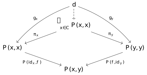
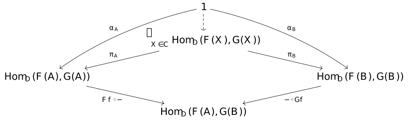
Theorem Vaughan (1977) [L3M8]
Rectangles, curves, and Klein bottles, related to Status of the smooth rectangular Peg problem
Every Jordan curve has an inscribed rectangle.
Theorem Nonexistence of an embedded Klein surface [local-0]
No continuous embedding of the Klein surface into . This is a standard result from algebraic topology. Using Alexander duality to compute homology, we produce a contradiction.
Proof [local-1]
Given a Jordan curve , the set of unordered and unequal pairs of points in , denoted , is an open Möbius band. Because every unequal unordered pair of points in the circle determines a unique point in : Take the two tangent lines to the circle at these points and intersect them.
If tangent lines are parallel, than it indicates the infinite point of :
Therefore, are the points of the complement of the closed unit disk in the projective plane, hence an open Möbius band.
Consider a map defined by
Geometrically, maps the ordered pair to a point encoding the midpoint of the segment (2D) and the length of the segment (1D).
If , then these four points form an inscribed rectangle. Hence we just need to prove that the map is not injective!
Consider where reflects the shape in the XY-plane. This is a Klein surface by gluing two Möbius strips at their boundary.
If is injective, then can be embedded into , which contradicts the theorem that nonexistence of an embedded Klein surface into .
Model mapping TT to untyped LC [ag-000Y]
{-# OPTIONS --without-K #-}
open import MLTT.Spartan hiding (Π; zero; succ)
open import UF.FunExt
open import ag-000V
open import ag-000W

module ag-000Y (fe : Fun-Ext) where
A model mapping TT to untyped lambda calculus.
module LC-TT {𝓤 𝓥 : Universe} (l : LC {𝓥}) where
  open LC
  open TT
  open TT-sorts
  open TT-ctors

  ex-sorts : TT-sorts {𝓤} {𝓥}
  ex-sorts .Ty = 𝟙
  ex-sorts .Tm _ = l .Λ

  ex-ctors : TT-ctors ex-sorts
  ex-ctors .Π A B = ⋆
  ex-ctors .lam f = l .lambda f
  ex-ctors .app f x = l .apply f x
  ex-ctors .lam-app = l .η _
  ex-ctors .app-lam {a}{b}{f} =
    (λ x → l .apply (l .lambda f) x) =⟨ dfunext fe (λ x → l .β f x) ⟩
    (λ x → f x) =⟨ refl ⟩
    f ∎
  ex-ctors .U = ⋆
  ex-ctors .El _ = ⋆
  ex-ctors .Nat = ⋆
  ex-ctors .zero = zeroΛ l
  ex-ctors .succ x = succΛ l x
  ex-ctors .elim-Nat X ze su n = recΛ l ze su n
  ex-ctors .elim-Nat-zero = recΛβ-zero l
  ex-ctors .elim-Nat-succ = recΛβ-succ l

  ex : TT {𝓤} {𝓥}
  ex .sorts = ex-sorts
  ex .ctors = ex-ctors
SOGAT of type theory with -types, a Tarski universe, and natural numbers [ag-000W]
Learn from https://github.com/kontheocharis/erasure-agda
{-# OPTIONS --safe --without-K --confluence-check #-}
module ag-000W where

open import MLTT.Spartan hiding (Π; zero; succ)

coe : {X X' : 𝓤 ̇ } → X = X' → X → X'
coe = transport id
TT 要用的 sorts,以及如果 Type 相等,可以轉換 term 用的 helper
coeTm
record TT-sorts : (𝓤 ⊔ 𝓥)⁺ ̇ where field Ty : 𝓤 ̇ Tm : Ty → 𝓥 ̇ coeTm : ∀ {A B : Ty} → A = B → Tm A → Tm B coeTm p a = coe (ap Tm p) a
TT 的 SOGAT
module _ (sorts : TT-sorts {𝓤} {𝓥}) where open TT-sorts sorts private variable A B C : Ty X Y Z : Tm _ → Ty t u v : Tm _ f g h : (a : Tm _) → Tm _ eq : _ = _ record TT-ctors : (𝓤 ⊔ 𝓥)⁺ ̇ where field -- Pi types Π : (A : Ty) → (Tm A → Ty) → Ty lam : ((a : Tm A) → Tm (X a)) → Tm (Π A X) app : Tm (Π A X) → (a : Tm A) → Tm (X a) lam-app : lam (app t) = t app-lam : app (lam f) = f -- Universe U : Ty El : Tm U → Ty -- Natural numbers Nat : Ty zero : Tm Nat succ : Tm Nat → Tm Nat elim-Nat : (X : Tm Nat → Ty) → (Tm (X zero)) → ((n : Tm Nat) → Tm (X n) → Tm (X (succ n))) → (n : Tm Nat) → Tm (X n) -- Computation for elim-Nat elim-Nat-zero : ∀ {mz ms} → elim-Nat X mz ms zero = mz elim-Nat-succ : ∀ {mz ms n} → elim-Nat X mz ms (succ n) = ms n (elim-Nat X mz ms n) record TT : (𝓤 ⊔ 𝓥)⁺ ̇ where field sorts : TT-sorts {𝓤} {𝓥} open TT-sorts sorts public field ctors : TT-ctors sorts open TT-ctors ctors public
Definition Riemann curvature tensor [B2D1]
The curvature of a Riemannian manifold is a tensor
where are vector fields, is the Levi-Civita connection of the metric (see Lectures on the Geometry of Manifolds Proposition 4.1.9.).
In local coordinates we have
In terms of the Christoffel symbols we have
Lowering the indices we have a new tensor
Theorem The Hairy Ball Theorem [DRE0]
用 constant vector field on plane 然後拉回 的定義方法很妙。
定理的證明是用 Flux 不變,但如果有處處非零的連續向量場,就可以讓 Flux 改變,矛盾。因此這樣的向量場不可能存在。
3-sphere (群 ) 跟 [JRT2]
用 quotient 掉 antipodal points 會得到 Real projective space 。
Proposition is not simple [local-1]
Proof [local-0]
因為 是 的 normal subgroup: 跟 for all 都還是屬於 。
而 nontrivial,有 nontrivial normal subgroup 的群 not simple
是群 :The group of rotations of 。 is simple 所以跟 不是同一個群
作為一個群可以視為 2x2 複數矩陣的群,元素為
這又稱為 The special unitary group 。
Definition Hopf bundle [5A3M]
Identify the unit odd dimensional sphere with the submanifold
an -action on given by
The complex projective space is isomorphic to , the group corresponds to . This quotient map is a principal bundle called Hopf bundle.
- by definition of
- Use (because , these describe all points in the projective space). The map defined by then
SOGAT of untyped lambda calculus [ag-000V]
{-# OPTIONS --safe --without-K #-} open import MLTT.Spartan hiding (id) open import ag-0005 module ag-000V where
SOGAT of untyped lambda calculus.
record LC : 𝓤 ⁺ ̇ where field Λ : 𝓤 ̇ lambda : (f : Λ → Λ) → Λ apply : Λ → Λ → Λ β : ∀ f x → apply (lambda f) x = f x η : ∀ f → lambda (λ x → apply f x) = f _$_ : Λ → Λ → Λ x $ y = apply x y infixl 30 _$_ syntax lambda (λ x → t) = ƛ x ⇒ t zeroΛ : Λ zeroΛ = ƛ z ⇒ ƛ s ⇒ z succΛ : Λ → Λ succΛ n = ƛ z ⇒ ƛ s ⇒ (s $ n $ (n $ z $ s)) id : Λ id = ƛ x ⇒ x recΛ : Λ → (Λ → Λ → Λ) → Λ → Λ recΛ zr su n = n $ zr $ (ƛ k ⇒ ƛ sk ⇒ su k sk) recΛβ-zero : ∀ {zr su} → recΛ zr su zeroΛ = zr recΛβ-zero {zr} {su} = (ap (_$ (ƛ k ⇒ ƛ sk ⇒ su k sk)) (β (λ z → ƛ s ⇒ z) zr)) ∙ (β (λ _ → zr) (ƛ k ⇒ ƛ sk ⇒ su k sk)) recΛβ-succ : ∀ {zr su n} → recΛ zr su (succΛ n) = su n (recΛ zr su n) recΛβ-succ {zr} {su} {n} = (ap (_$ (ƛ k ⇒ ƛ sk ⇒ su k sk)) (β (λ z → ƛ s ⇒ (s $ n $ (n $ z $ s))) zr)) ∙ (β (λ s → s $ n $ (n $ zr $ s)) (ƛ k ⇒ ƛ sk ⇒ su k sk)) ∙ (ap (_$ (n $ zr $ (ƛ k ⇒ ƛ sk ⇒ su k sk))) (β (λ k → ƛ sk ⇒ su k sk) n)) ∙ (β (λ sk → su n sk) (n $ zr $ (ƛ k ⇒ ƛ sk ⇒ su k sk))) embed-nat : ℕ → Λ embed-nat 0 = zeroΛ embed-nat (succ x) = succΛ (embed-nat x)
Lambda calculus (Second-order algebraic theories) universe polymorphic extended.
代數幾何:視 base ring 的元素為函數 [WYCP]
在 manifold 上我們可以定義 。在代數幾何裡面我們想要抽象並仿造這個結構,所以若 為一點(亦同時是 prime ideal),residue field at point 定義為 the field of fractions of the quotient ring
那麼,每個 取 將使 可以被視為一個「函數」,不過在不同點 的 codomain 都不同。構造即取 再取 。
Status of the smooth rectangular Peg problem [VEYQ]
https://www.math.columbia.edu/~ums/Peg%20problem%20-%20slides.pdf
- Emch (1913) solved the problem for smooth convex curves. (Proof uses configuration spaces and homology.)
- Schnirelman (1929) solved it for any smooth Jordan curve.
Theorem Vaughan (1977) [local-0]
Every continuous Jordan curve contains four points forming the vertices of some rectangle. This is what 3b1b did, see video here.
Theorem Greene-Lobb (2020) [local-1]
Given a smooth Jordan curve and a rectangle in the plane, then contain four points forming the vertices of a rectangle similar to R.
Theorem Barr's theorem [KGRZ]
If is a Grothendieck topos, then there is a surjective geometric morphism
where satisfies the axiom of choice.
presheaves exponential 同構的推導 [21ME]
Topos Theory 的 1.12
令 為 category 的 presheaves,那麼
Proof [local-0]
- 用 Presheaves are colimits of representables 改寫
- Contravariant 用到的是 Hom-functors preserve limits
Proposition Hom-functors preserve limits [math-TGEI]
This is a very useful property of hom-functor.
Let be a category, then its hom-functor can be wrote as
If the limit exists in , then for all there is a natural isomorphism
If the colimit exists in , then for all there is a natural isomorphism
See nLab for more details.
Definition Holonomy [math-L2W1]
Let be a vector bundle with a connection . The holonomy of along a closed path is the parallel transport along .
Definition Parallel transport [math-XU4I]
Let be a vector bundle with a connection . For any smooth path we will define a linear isomorphism called the parallel transport along .
The construction [local-0]
More precisely, we construct a family of linear isomorphisms:
for all . Consider arbitrary , let be a vector, then define , we know . What we are searching is a "constant" path, in the sense that derivative is , hence we want
so this suggests a way of defining : For any and any , define as the value at of the solution of the initial value problem:
And this is a system of linear ordinary differential equations in disguise.
Definition Covariant Derivative (Linear Connection) [math-HCIJ]
Let be a vector bundle. A covariant derivative on is a -linear map
such that, for all and all , we have
where denotes the space of smooth sections of over .
Remind that
Therefore, has a more traditional view
When a map is an equivalence? [RNNM]
For a given function , the following are two correct definitions of f is an equivalence.
Defintion Voevodsky's [ag-000T]
is an equivalence if its fibers are contractible (or singletons): For every , the type
fiber : {X : 𝓤 ̇ } {Y : 𝓥 ̇ } → (X → Y) → Y → 𝓤 ⊔ 𝓥 ̇ fiber f y = Σ x ꞉ domain f , f x = y
has the property that there is a distinguished element such that for all .
is-equiv : {X : 𝓤 ̇ } {Y : 𝓥 ̇ } → (f : X → Y) → 𝓤 ⊔ 𝓥 ̇ is-equiv f = ∀ (y : codomain f) → Σ σ₀ ꞉ fiber f y , ∀ (σ : fiber f y) → σ = σ₀
Defintion Joyal's [ag-000U]
is an equivalence if it has a section and also has a retraction:
{-# OPTIONS --safe --without-K #-} module ag-000U where open import MLTT.Spartan open import UF.Base open import UF.Sets open import UF.Sets-Properties
is-equiv : {X : 𝓤 ̇ } {Y : 𝓥 ̇ } → (f : X → Y) → 𝓤 ⊔ 𝓥 ̇ is-equiv f = (Σ s ꞉ (codomain f → domain f) , f ∘ s ∼ id) × (Σ r ꞉ (codomain f → domain f) , r ∘ f ∼ id)
Of course, the second post in thread is more important, there is a wrong definition, and Escardo shows why it's wrong.
什麼是量子幾何 [FWA9]
Why , A Four Dimensional Proof [E963]
JIT: Write XOR Execute policy [UIC7]
所謂的 W^X (Write XOR Execute) policy 是指不要讓記憶體同時是 PROT_WRITE 跟 PROT_EXEC,所以正確的配置方式是(參見 mmap)
- 先設定成
PROT_READ | PROT_WRITE - 等寫完指令再改成
PROT_READ | PROT_EXEC(像是用mprotecthttps://man7.org/linux/man-pages/man2/mprotect.2.html)
然後才能真的執行這段程式。
Corollary About Boolean ring [math-HS0H]
Let be a Boolean ring (see nLab) and .
Tool Unsure Calculator [VIPY]
Theorem The field of fractions is a torsion-free module [math-3E35]
Let be an integral domain, and is the field of fractions of . Then is a torsion-free -module (see The Stacks project tag/0549).
Proof [local-0]
We want to show that the only torsion element of is . Every element of has the form where , now suppose is a torsion. Then there exists a such that
which leads
in an integral domain, this leads or , but by definition, hence . Which means is , be torsion is be zero in , is a torsion-free -module.
Theorem Premanifold 為 Hausdorff 的等價條件 [math-T4B3]
令 為一個 premanifold(field 為 或是 )。則以下條件等價:
- 為 Hausdorff 空間
- 對於 中任意相異兩點 (),存在開集 使得 ,且在 中,存在函數 使得
Proof [local-0]
(2) ⇒ (1):設 為相異兩點。由條件 (2),存在開集 使得 ,且存在 使得 。
令 。因為 為 smooth 函數,存在 的開鄰域 使所有 ,有 。
同理,存在 的開鄰域 使得對所有 ,有 。於是我們知道 ,因為如果存在 ,則:
為矛盾,也就是說不存在這種 。因此 為 Hausdorff 空間。
(1) ⇒ (2):設 為相異兩點。因為 為 Hausdorff 空間,存在不相交的開鄰域 和 使得 。
因為 為 premanifold,存在 open cover 使得每個 與某個 local ringed space 同構。因此存在 和 使得 且 。
考慮開集 和 。因為 ,我們有 。
取 的開鄰域 及函數 使得 (此函數對應於 stalk 的 maximal ideal 中的元素)。同理,取 的開鄰域 及函數 使得 (對應於 stalk 中不在 maximal ideal 的元素)。
令 ,則 為開集且 。因 與 不相交,可定義函數 ,在 上取 ,在 上取 。於是 而 , 與 滿足條件 (2)。
NOTE: Explicit Weakening [ag-000S]
在 Substitution Without Copy and Paste 結尾也有提過這篇,就來稍微看一下。
Explicit Weakening
{-# OPTIONS --rewriting --no-level-universe #-} module ag-000S where open import MLTT.Spartan hiding (Type; id) {-# BUILTIN REWRITE _=_ #-} cong₂ : ∀ {A B C : 𝓤 ̇ } (f : A → B → C) {x y u v} → x = y → u = v → f x u = f y v cong₂ f refl refl = refl
data Type : 𝓤₀ ̇ where base : Type _⇒_ : Type → Type → Type infixr 7 _⇒_ variable A B C : Type data Con : 𝓤₀ ̇ where ∅ : Con _▷_ : Con → Type → Con infixl 5 _▷_ variable Γ Δ Θ Ξ : Con data _⊢_ : Con → Type → 𝓤₀ ̇ where • : Γ ▷ A ⊢ A _↑ : (M : Γ ⊢ B) ------------ → Γ ▷ A ⊢ B ƛ_ : (N : Γ ▷ A ⊢ B) → Γ ⊢ A ⇒ B _·_ : (L : Γ ⊢ A ⇒ B) (M : Γ ⊢ A) ----------------------------- → Γ ⊢ B infix 5 ƛ_ infix 4 _⊢_ infixl 7 _·_ variable L M N P Q : Γ ⊢ A data _⊨_ : Con → Con → 𝓤₀ ̇ where id : Δ ⊨ Δ _↑ : (σ : Γ ⊨ Δ) → Γ ▷ A ⊨ Δ _▷_ : (σ : Γ ⊨ Δ) (M : Γ ⊢ A) ------------ → Γ ⊨ Δ ▷ A infix 4 _⊨_ infix 8 _↑ variable σ τ υ : Γ ⊨ Δ pattern △ = _ ▷ _
Instantiation
_[_] : (M : Δ ⊢ A) (σ : Γ ⊨ Δ) → Γ ⊢ A M [ id ] = M M [ σ ↑ ] = (M [ σ ]) ↑ • [ σ ▷ P ] = P (M ↑) [ σ ▷ P ] = M [ σ ] (ƛ M) [ σ @ △ ] = ƛ (M [ σ ↑ ▷ • ]) (L · M) [ σ @ △ ] = L [ σ ] · (M [ σ ]) _⨟_ : (σ : Θ ⊨ Δ) (τ : Γ ⊨ Θ) → Γ ⊨ Δ σ ⨟ id = σ σ ⨟ (τ ↑) = (σ ⨟ τ) ↑ id ⨟ τ @ △ = τ (σ ↑) ⨟ (τ ▷ Q) = σ ⨟ τ (σ ▷ P) ⨟ τ @ △ = (σ ⨟ τ) ▷ (P [ τ ]) infixl 5 _⨟_ [][] : (M : Δ ⊢ A) (σ : Θ ⊨ Δ) (τ : Γ ⊨ Θ) → M [ σ ] [ τ ] = M [ σ ⨟ τ ] [][] M σ id = refl [][] M σ (τ ↑) = ap _↑ ([][] M σ τ) [][] M id (τ ▷ M₁) = refl [][] M (σ ↑) (τ ▷ M₁) = [][] M σ τ [][] • (σ ▷ P) τ@△ = refl [][] (M ↑) (σ ▷ P) τ@△ = [][] M σ τ [][] (ƛ N) σ@△ τ@△ = ap ƛ_ ([][] N (σ ↑ ▷ •) (τ ↑ ▷ •)) [][] (L · M) σ@△ τ@△ = cong₂ _·_ ([][] L σ τ) ([][] M σ τ) {-# REWRITE [][] #-}
Left identity
left-id : (τ : Γ ⊨ Δ) → id ⨟ τ = τ left-id id = refl left-id (τ ↑) = ap _↑ (left-id τ) left-id (τ ▷ Q) = refl {-# REWRITE left-id #-}
Associative
assoc : (σ : Θ ⊨ Δ) (τ : Ξ ⊨ Θ) (υ : Γ ⊨ Ξ) → (σ ⨟ τ) ⨟ υ = σ ⨟ (τ ⨟ υ) assoc σ τ id = refl assoc σ τ (υ ↑) = ap _↑ (assoc σ τ υ) assoc σ id (υ ▷ M) = refl assoc σ (τ ↑) (υ ▷ M) = assoc σ τ υ assoc id (τ ▷ M₁) (υ ▷ M) = refl assoc (σ ↑) (τ ▷ M₁) (υ ▷ M) = assoc σ τ (υ ▷ M) assoc (σ ▷ M₂) (τ ▷ M₁) (υ ▷ M) = cong₂ _▷_ (assoc σ (τ ▷ M₁) (υ ▷ M)) refl {-# REWRITE assoc #-}
下面的案例是本來在 PLFA 中不好做出來,但用這套就很簡單的問題
_[_]₀ : (N : Γ ▷ A ⊢ B) (M : Γ ⊢ A) ------------ → Γ ⊢ B N [ M ]₀ = N [ id ▷ M ] _[_]₁ : (N : Γ ▷ A ▷ B ⊢ C) (M : Γ ⊢ A) ------------ → Γ ▷ B ⊢ C N [ M ]₁ = N [ (id ▷ M) ↑ ▷ • ] double-subst : N [ M ]₁ [ L ]₀ = N [ L ↑ ]₀ [ M ]₀ double-subst = refl commute-subst : N [ M ]₀ [ L ]₀ = N [ L ]₁ [ M [ L ]₀ ]₀ commute-subst = refl
最後也有談到缺點是 identifying when terms are equivalent may become more difficult,但我沒有試這是什麼清況。
NOTE: Substitution Without Copy and Paste [tt-IHCF]
Substitution Without Copy and Paste
The copy-and-paste approach [ag-000M]
{-# OPTIONS --safe --without-K #-} module ag-000M where open import MLTT.Spartan
類型跟 context
data Ty : 𝓤₀ ̇ where base : Ty _⇒_ : Ty → Ty → Ty infixl 50 _⇒_ data Con : 𝓤₀ ̇ where ◇ : Con _▷_ : Con → Ty → Con infixl 40 _▷_
- 等一下用的變數
- de Bruijn variables
- terms
variable Γ Δ Ξ : Con A B C : Ty data _∋_ : Con → Ty → 𝓤₀ ̇ where here : Γ ▷ A ∋ A there : Γ ∋ A → (B : Ty) ------------------ → Γ ▷ B ∋ A infixl 30 _∋_ data _⊢_ : Con → Ty → 𝓤₀ ̇ where -- embeds variables in λ-terms `_ : Γ ∋ A → Γ ⊢ A -- application t · u _·_ : Γ ⊢ A ⇒ B → Γ ⊢ A → Γ ⊢ B ƛ_ : Γ ▷ A ⊢ B → Γ ⊢ A ⇒ B infixl 20 _⊢_ infixl 60 `_ infixl 50 _·_ infixl 40 ƛ_
substitution 定義成
data _⊩_ : Con → Con → 𝓤₀ ̇ where ε : Γ ⊩ ◇ _,_ : Γ ⊩ Δ → Γ ⊢ A → Γ ⊩ Δ ▷ A
現在要定義 substitution 在 terms 跟 variables 上的作用:
_v[_] : Δ ∋ A → Γ ⊩ Δ → Γ ⊢ A here v[ ts , t ] = t there i B v[ ts , t ] = i v[ ts ] data _⊩v_ : Con → Con → 𝓤₀ ̇ where ε : Γ ⊩v ◇ _,_ : Γ ⊩v Δ → Γ ∋ A → Γ ⊩v Δ ▷ A _v[_]v : Γ ∋ A → Δ ⊩v Γ → Δ ∋ A here v[ is , i ]v = i there i B v[ is , j ]v = i v[ is ]v _⁺v_ : Γ ⊩v Δ → (A : Ty) → Γ ▷ A ⊩v Δ ε ⁺v A = ε (is , i) ⁺v A = (is ⁺v A) , there i A _↑v_ : Γ ⊩v Δ → (A : Ty) → Γ ▷ A ⊩v Δ ▷ A is ↑v A = (is ⁺v A) , here _[_]v : Γ ⊢ A → Δ ⊩v Γ → Δ ⊢ A (` i) [ is ]v = ` (i v[ is ]v) (t · u) [ is ]v = (t [ is ]v) · (u [ is ]v) (ƛ t) [ is ]v = ƛ (t [ is ↑v _ ]v) idv : Γ ⊩v Γ idv {Γ = ◇} = ε idv {Γ = Γ ▷ A} = idv ↑v A
為了定義下面的 suc-tm,需要定義上面大量的類似結構
Γ ⊩v Δ
_⁺_ : Γ ⊩ Δ → (A : Ty) → Γ ▷ A ⊩ Δ ε ⁺ A = ε (ts , t) ⁺ A = (ts ⁺ A) , suc-tm t A where suc-tm : Γ ⊢ B → (A : Ty) → Γ ▷ A ⊢ B suc-tm t A = t [ idv ⁺v A ]v _↑_ : Γ ⊩ Δ → (A : Ty) → Γ ▷ A ⊩ Δ ▷ A ts ↑ A = ts ⁺ A , ` here _[_] : Γ ⊢ A → Δ ⊩ Γ → Δ ⊢ A (` i) [ ts ] = i v[ ts ] (t · u) [ ts ] = (t [ ts ]) · (u [ ts ]) (ƛ t) [ ts ] = ƛ (t [ ts ↑ _ ])
所以為了避免這些重複,方法要改成:
Substituion without copy and paste 的提議 [ag-000N]
{-# OPTIONS --safe --without-K #-} module ag-000N where open import MLTT.Spartan hiding (_⊔_; id) open import ag-000M using (Ty; _⇒_; Con; ◇; _▷_) variable Γ Δ Ξ : Con A B C : Ty
引入 Sort 區分 variable 跟 term 的情況
mutual data Sort : 𝓤₀ ̇ where V : Sort T>V : (s : Sort) → IsV s → Sort data IsV : Sort → 𝓤₀ ̇ where isV : IsV V pattern T = T>V V isV variable q r s : Sort
這樣就可以把 variables 跟 terms 定義到一起,用 s 區分
Γ ⊢[ s ] A 是 variable 還是 term
data _⊢[_]_ : Con → Sort → Ty → 𝓤₀ ̇ where here : Γ ▷ A ⊢[ V ] A there : Γ ⊢[ V ] A → (B : Ty) → Γ ▷ B ⊢[ V ] A `_ : Γ ⊢[ V ] A → Γ ⊢[ T ] A _·_ : Γ ⊢[ T ] A ⇒ B → Γ ⊢[ T ] A → Γ ⊢[ T ] B ƛ_ : Γ ▷ A ⊢[ T ] B → Γ ⊢[ T ] A ⇒ B variable x y z : Γ ⊢[ q ] A
substitution 現在定義成
data _⊩[_]_ : Con → Sort → Con → 𝓤₀ ̇ where ε : Γ ⊩[ q ] ◇ _,_ : Γ ⊩[ q ] Δ → Γ ⊢[ q ] A → Γ ⊩[ q ] Δ ▷ A variable xs ys zs : Δ ⊩[ q ] Γ
現在需要考慮 sort 之間的關係,這些 lemma 有助於簡化後面的證明
data _⊑_ : Sort → Sort → Set where rfl : s ⊑ s v⊑t : V ⊑ T _⊔_ : Sort → Sort → Sort V ⊔ r = r T ⊔ r = T
一些輔助用的 REWRITE [ag-000O]
{-# OPTIONS --without-K --rewriting #-} module ag-000O where open import MLTT.Spartan hiding (_⊔_; id) open import ag-000M using (Ty; _⇒_; Con; ◇; _▷_) open import ag-000N {-# BUILTIN REWRITE _=_ #-}
這邊的定義很繁瑣但只是單純攤開 V、T
就能證明,並不是很重要。重點在最後用 REWRITE
避免後續需要證明一些麻煩的情況
⊑t : s ⊑ T ⊑t {V} = v⊑t ⊑t {T} = rfl v⊑ : V ⊑ s v⊑ {V} = rfl v⊑ {T} = v⊑t ⊑q⊔ : q ⊑ (q ⊔ r) ⊑q⊔ {V}{V} = rfl ⊑q⊔ {V}{T} = v⊑t ⊑q⊔ {T}{V} = rfl ⊑q⊔ {T}{T} = rfl ⊔⊔ : q ⊔ (r ⊔ s) = (q ⊔ r) ⊔ s ⊔⊔ {V}{V}{V} = refl ⊔⊔ {V}{V}{T} = refl ⊔⊔ {V}{T}{V} = refl ⊔⊔ {V}{T}{T} = refl ⊔⊔ {T}{V}{V} = refl ⊔⊔ {T}{V}{T} = refl ⊔⊔ {T}{T}{V} = refl ⊔⊔ {T}{T}{T} = refl ⊔v : q ⊔ V = q ⊔v {V} = refl ⊔v {T} = refl ⊔t : q ⊔ T = T ⊔t {V} = refl ⊔t {T} = refl ⊑⊔r : r ⊑ (q ⊔ r) ⊑⊔r {V}{V} = rfl ⊑⊔r {V}{T} = v⊑t ⊑⊔r {T}{V} = rfl ⊑⊔r {T}{T} = rfl ⊔-self : q ⊔ q = q ⊔-self {V} = refl ⊔-self {T} = refl {-# REWRITE ⊔⊔ ⊔v ⊔t ⊔-self #-}
substitution 的組合 [ag-000P]
{-# OPTIONS --without-K --rewriting #-} module ag-000P where open import MLTT.Spartan hiding (_⊔_; id) open import ag-000M using (Ty; _⇒_; Con; ◇; _▷_) open import ag-000N open import ag-000O
這裡的目的是定義 ⊑ relation 對 term 的影響,以及定義
substitution 的結合 ◦
tm⊑ : q ⊑ s → Γ ⊢[ q ] A → Γ ⊢[ s ] A tm⊑ rfl x = x tm⊑ v⊑t i = ` i here[_] : (q : Sort) → Γ ▷ A ⊢[ q ] A here[ V ] = here here[ T ] = ` here mutual _[_] : Γ ⊢[ q ] A → Δ ⊩[ r ] Γ → Δ ⊢[ q ⊔ r ] A here [ xs , x ] = x there i _ [ xs , x ] = i [ xs ] (` i) [ xs ] = tm⊑ ⊑t (i [ xs ]) (t · u) [ xs ] = (t [ xs ]) · (u [ xs ]) (ƛ t) [ xs ] = ƛ (t [ xs ↑ _ ]) id-poly : (q : Sort) → Γ ⊩[ q ] Γ id-poly {Γ = ◇} q = ε id-poly {Γ = Γ ▷ A} q = id-poly q ↑ A id : Γ ⊩[ V ] Γ id = id-poly V {-# INLINE id #-} there[_] : (q : Sort) → Γ ⊢[ q ] B → (A : Ty) → Γ ▷ A ⊢[ q ] B there[ V ] i A = there i A there[ T ] t A = t [ id ⁺ A ] _⁺_ : Γ ⊩[ q ] Δ → (A : Ty) → Γ ▷ A ⊩[ q ] Δ ε ⁺ A = ε (ts , t) ⁺ A = (ts ⁺ A) , there[ _ ] t A _↑_ : Γ ⊩[ q ] Δ → (A : Ty) → Γ ▷ A ⊩[ q ] Δ ▷ A ts ↑ A = ts ⁺ A , here[ _ ] infixl 70 _⁺_ _◦_ : Γ ⊩[ q ] Ξ → Δ ⊩[ r ] Γ → Δ ⊩[ q ⊔ r ] Ξ ε ◦ ys = ε (xs , x) ◦ ys = (xs ◦ ys) , x [ ys ]
Proposition The right identity law [ag-000Q]
{-# OPTIONS --without-K --rewriting #-} module ag-000Q where open import MLTT.Spartan hiding (_⊔_; id) open import ag-000M using (Ty; _⇒_; Con; ◇; _▷_) open import ag-000N open import ag-000O open import ag-000P
⁺-nat[]v : (i : Γ ⊢[ V ] A) → (xs : Δ ⊩[ q ] Γ) → i [ xs ⁺ B ] = there[ q ] (i [ xs ]) B ⁺-nat[]v here (xs , x) = refl ⁺-nat[]v (there j _) (xs , x) = ⁺-nat[]v j xs [id] : x [ id ] = x [id] {x = here} = refl [id] {x = there i B} = (i [ id ⁺ B ]) =⟨ ⁺-nat[]v {q = V} i id ⟩ there (i [ id ]) B =⟨ ap (λ - → there - B) [id] ⟩ there i B ∎ [id] {x = ` i} = ap `_ [id] [id] {x = t · u} = ((t [ id ]) · (u [ id ])) =⟨ ap (t [ id ] ·_) [id] ⟩ ((t [ id ]) · u) =⟨ ap (_· u) [id] ⟩ (t · u) ∎ [id] {x = ƛ t} = ap ƛ_ [id] ◦id : xs ◦ id = xs ◦id {xs = ε} = refl ◦id {xs = xs , x} = (xs ◦ id) , (x [ id ]) =⟨ ap ((xs ◦ id) ,_) [id] ⟩ (xs ◦ id) , x =⟨ ap (_, x) ◦id ⟩ xs , x ∎
Proposition Left identity law 與 Associative law [ag-000R]
{-# OPTIONS --allow-unsolved-metas --without-K --rewriting #-} module ag-000R where open import MLTT.Spartan hiding (_⊔_; id) open import ag-000M using (Ty; _⇒_; Con; ◇; _▷_) open import ag-000N open import ag-000O open import ag-000P open import ag-000Q
這兩個是 mutual 定義的,而且有一些 goals 我也看不出怎麼解了,暫時就先這樣 xd
tm[] : tm⊑ ⊑t (x [ xs ]) = (tm⊑ ⊑t x) [ xs ] tm[] {x = here} = refl tm[] {x = there x B} = refl tm[] {x = ` x} = tm[] {x = x} tm[] {x = x · x₁} = refl tm[] {x = ƛ x} = refl zero[] : {q : Sort} {r : Sort} {Γ : Con} {Δ : Con} {A : Ty} {xs : Δ ⊩[ r ] Γ} {x : Δ ⊢[ r ] A} → here[ q ] [ xs , x ] = tm⊑ (⊑⊔r {q = q}) x zero[] {q = V} {r = V} = refl zero[] {q = V} {r = T} = refl zero[] {q = T} {r = V} = refl zero[] {q = T} {r = T} = refl tm⊑zero : (q⊑r : q ⊑ r) → here[ r ] = tm⊑ q⊑r here[ q ] tm⊑zero rfl = refl tm⊑zero v⊑t = refl {-# TERMINATING #-} mutual suc[] : (there[ s ] x _) [ ys , y ] = x [ ys ] suc[] {s = V} = refl suc[] {s = T} {x = x} {ys = ys} {y = y} = there[ T ] x _ [ ys , y ] =⟨ refl ⟩ x [ id ⁺ _ ] [ ys , y ] =⟨ [◦] {x = x} ⁻¹ ⟩ x [ (id ⁺ _) ◦ (ys , y) ] =⟨ ap (x [_]) ⁺◦ ⟩ x [ id ◦ ys ] =⟨ ap (x [_]) id◦ ⟩ x [ ys ] ∎ ⁺◦ : xs ⁺ A ◦ (ys , x) = xs ◦ ys ⁺◦ {xs = ε} = refl ⁺◦ {xs = ts , t} {A = A} {ys = ys} {x = x} = ((ts ⁺ A) ◦ (ys , x)) , (there[ _ ] t A [ ys , x ]) =⟨ ap (((ts ⁺ A) ◦ (ys , x)) ,_) (suc[] {x = t}) ⟩ ((ts ⁺ A) ◦ (ys , x)) , (t [ ys ]) =⟨ ap (_, (t [ ys ])) ⁺◦ ⟩ (ts ◦ ys) , (t [ ys ]) ∎ ⁺−nat◦ : {xs : Δ ⊩[ q ] Γ} → {ys : Ξ ⊩[ r ] Δ} → {A : Ty} → xs ◦ (ys ⁺ A) = (xs ◦ ys) ⁺ A ⁺−nat◦ {xs = ε} = refl ⁺−nat◦ {q = q} {r = r} {xs = xs , x} {ys = ys} {A = A} = (xs ◦ (ys ⁺ A)) , (x [ ys ⁺ A ]) =⟨ ap ((xs ◦ (ys ⁺ A)) ,_) (⁺-nat[] {q = q} {B = A} {x = x} {xs = ys}) ⟩ (xs ◦ (ys ⁺ A)) , there[ _ ] (x [ ys ]) A =⟨ ap (_, there[ _ ] (x [ ys ]) A) ⁺−nat◦ ⟩ ((xs ◦ ys) ⁺ A) , there[ _ ] (x [ ys ]) A ∎ ⁺-nat[] : {q r : Sort} → {A B : Ty} → {x : Γ ⊢[ q ] A} → {xs : Δ ⊩[ r ] Γ} → x [ xs ⁺ B ] = there[ q ⊔ r ] (x [ xs ]) B ⁺-nat[] {q = V} {x = i} {xs = xs} = ⁺-nat[]v i xs ⁺-nat[] {q = T} {B = B} {x = x} {xs = xs} = x [ xs ⁺ B ] =⟨ ap (λ - → x [ - ⁺ B ]) (◦id {xs = xs} ⁻¹) ⟩ x [ (xs ◦ id) ⁺ B ] =⟨ ap (x [_]) (⁺−nat◦ ⁻¹) ⟩ x [ xs ◦ (id ⁺ B) ] =⟨ [◦] {x = x} ⟩ x [ xs ] [ id ⁺ B ] =⟨ refl ⟩ there[ T ] (x [ xs ]) B ∎ ↑◦ : {r s : Sort} → {xs : Δ ⊩[ r ] Ξ} → {ys : Γ ⊩[ s ] Δ} → {A : Ty} → (xs ◦ ys) ↑ A = (xs ↑ A) ◦ (ys ↑ A) ↑◦ {r = r} {s = s} {xs = xs} {ys = ys} {A = A} = (xs ◦ ys) ↑ A =⟨ refl ⟩ (xs ◦ ys) ⁺ A , here[ r ⊔ s ] =⟨ ap (λ - → - , here[ _ ]) (⁺−nat◦ ⁻¹) ⟩ xs ◦ (ys ⁺ A) , here[ r ⊔ s ] =⟨ ap (xs ◦ (ys ⁺ A) ,_) (tm⊑zero (⊑⊔r {r = s} {q = r})) ⟩ xs ◦ (ys ⁺ A) , tm⊑ (⊑⊔r {q = r}) here[ s ] =⟨ ap (xs ◦ (ys ⁺ A) ,_) (zero[] {q = r} {r = s} {A = A} {xs = ys ⁺ A} {x = here[ s ]} ⁻¹) ⟩ xs ◦ (ys ⁺ A) , (here[ r ] [ ys ↑ A ]) =⟨ ap (_, (here[ r ] [ ys ↑ A ])) (⁺◦ {xs = xs} {A = A} {ys = ys ⁺ A} {x = here[ s ]} ⁻¹) ⟩ ((xs ⁺ A) ◦ (ys ⁺ A , here[ s ])) , (here[ r ] [ ys ↑ A ]) =⟨ refl ⟩ (xs ↑ A) ◦ (ys ↑ A)∎ [◦] : x [ xs ◦ ys ] = x [ xs ] [ ys ] [◦] {x = here} {xs = xs , x} = refl [◦] {x = there i B} {xs = xs , x} = [◦] {x = i} [◦] {x = ` x} {xs = xs} {ys = ys} = tm⊑ ⊑t (x [ xs ◦ ys ]) =⟨ ap (λ - → tm⊑ ⊑t -) ([◦] {x = x}) ⟩ tm⊑ ⊑t (x [ xs ] [ ys ]) =⟨ tm[] {x = x [ xs ]} ⟩ (tm⊑ ⊑t (x [ xs ]) [ ys ]) ∎ [◦] {x = t · u} {xs = xs} {ys = ys} = (t [ xs ◦ ys ]) · (u [ xs ◦ ys ]) =⟨ ap (_· (u [ xs ◦ ys ])) ([◦] {x = t}) ⟩ (t [ xs ] [ ys ]) · (u [ xs ◦ ys ]) =⟨ ap ((t [ xs ] [ ys ]) ·_) ([◦] {x = u}) ⟩ ((t [ xs ]) [ ys ]) · ((u [ xs ]) [ ys ]) ∎ [◦] {x = ƛ t} {xs = xs} {ys = ys} = ap ƛ_ (t [ (xs ◦ ys) ↑ _ ] =⟨ ap (t [_]) (↑◦ {xs = xs}) ⟩ t [ (xs ↑ _) ◦ (ys ↑ _) ] =⟨ [◦] {x = t} ⟩ (t [ xs ↑ _ ]) [ ys ↑ _ ] ∎) id◦' : Sort → id ◦ xs = xs id◦' {xs = ε} q = refl id◦' {xs = xs , x} q = ap (_, x) (((id ⁺ _) ◦ (xs , x)) =⟨ ⁺◦ ⟩ id ◦ xs =⟨ id◦ ⟩ xs ∎) id◦ : id ◦ xs = xs id◦ = id◦' V {-# INLINE id◦ #-}
到這裡已經證明了 contexts 與 substitutions 真的是一個範疇,而且這個範疇有 terminal object。第五節是把這邊的工作放進去 CwF-simple(constant presheaves 可以讓 CwF 適用於 simply typed calculus)裡,那個我暫時沒什麼興趣。
AI Is Slowly Destroying Your Brain [45VG]
新增一些心理學研究結果作為思考現代 - 商業、科技與政治交織的空間的案例。
Lie 群的意義 [VQ6V]
Lie 群是同時是群跟流形的物件,但這有什麼意義呢?
最簡單的案例是平面旋轉群 ,這是由所有平面上的旋轉組成的群,如果把所有的軌跡都畫到平面上,那這會構成一個 。而我們知道局部的看 可以視為一個直線(切線),這就使得局部的來說,可以用切線近似的討論,這條線被稱為 Lie algebra。
所以我們成功地把曲線問題變成線性問題,更重要的是,這個方法更廣泛來說還是有用,比如很多物理學研究的對稱性可以用某個 Lie 群研究。
另外很有趣的是,Complex number 除了可以用代數的方式定義(see Algebra: Chapter 0, III, Proposition 4.6.):
在 Naive Lie Theory 中提到我們也能用旋轉矩陣來定義。
Lawvere-Tierney topology [math-MRL4]
Let be a topos. A Lawvere-Tierney topology in is a morphism such that the following diagrams are commutative:
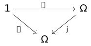
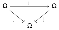
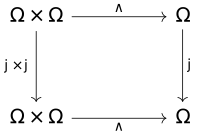
A topology in a topos gives rise to a new topos defined over .
Tool x86-64 Playground [software-9JPJ]
Definition Weil algebra [math-T4B2]
A Weil algebra is an algebra over the rational numbers , equipped with a morphism
such that is a local ring with maximal ideal:
with a nilpotent ideal, and such that is a finite dimensional -vector space.
The notion of Weil algebra makes sense in any topos with a natural numbers object .
Proposition nilpotent maps form a prime ideal [math-6W2V]
Definition Coprimary [local-0]
Let be a Noetherian ring. A nonzero finitely generated -module is coprimary if for all , the multiplication map (reuse element to denote it)
is injective or nilpotent.
If is coprimary, then the set
forms a prime ideal in .
Proof [local-1]
To check is a prime ideal, we want to check that if and then .
Because is coprimary, so such are injective, and
the composition of injective maps is injective, hence . □
具體的 Sheaf 以及如何得到 ringed 與 locally ringed space 的定義 [UXEP]
Sheaf 的定義是
Definition Sheaf [math-PPAW]
我們說一個 presheaf 是 sheaf 是指:對所有 open sets in 與所有 的 open covering ,以下兩個條件成立
- Let with for all . Then .
- Given for all such that for all . Then there exists an such that (注意,根據條件一這個 是唯一的)
對我個人比較有意義的案例是
Example 上的可微分函數 [local-0]
假設 是一個 -manifold(),我們通常用 表示集合
,而 是 的一個開集。這時候 是一個 sheaf of -algebras on
- 這本身也是一個 Ring
- 在這個案例中,stalk 也就變成經典的 function germs(用重合定義的函數局部等價類)。
所以 ringed space 也就定義成了
Definition Ringed space [math-9M06]
Ringed space 是一個 pair
- 一個 topological space
- 一個 sheaf of (commutative) rings
注意到如果 是一個 commutative ring,那 -algebra 也能視為一個 ring (with unit),所以這確實是 manifold 的推廣。
如果進一步要求 的每個 stalk 都是 local ring,那就得到了 locally ringed space:
Definition Locally Ringed space [math-AYGI]
Locally ringed space 是 ringed space 加上條件:for all
是一個 local ring(i.e. 有 maximal ideal)
語法作為一種檢視方式 [32PV]
正如 Bicameral, Not Homoiconic 一文所述(推薦先看完 Bicameral 再看我這裡寫的東西),真正讓 LISP 脫穎而出的功能,是它 pipeline 特殊的雙層解析器:
- scan 出詞素(token)
- 用 reader 讀出「資料」,通常是一種 form,以 LISP 來說就是 s-expression。而且 reader 會順便讀取 macro 定義跟把 macro 展開
- 最後用 parser 解析成表面語言
程式語言的設計會影響實現,有些實現方式會非常多的靜態檢查,以至於在這些實現內部消除了絕大多數的語意錯誤,像是 dependent typed 的語言,這時候我們幾乎可以相信這些編譯器的內部表示,跟我們等下提到的客觀語法真的一樣。要注意這並不總是成立,也有很多語意錯誤會被延遲到執行時再處理(如 Python、Racket 的情況),所以在程式語言的實現中,總是假設並依賴一個理想的客觀語法,是由我們規定的語意生成的,我們通常用化簡語意或是指稱語意去研究它,而編譯器很大一部分工作就是保證自己遵循這個語意來實現語言。一套客觀語法可以有很多種檢視方式,比如「指定 a 的新值是整數 1」這個客觀語法可以寫成
- Racket
(set-box! a 1) - C
a = 1; - OCaml
a := 1
更瘋狂一點的話,也不是不能寫成 JSON
{
"assign": {
"variable": "a",
"expression": {
"type": "int",
"val": 1
}
}
}
為什麼表面語法有可能是錯的呢?比如 OCaml 的 parser 不會拒絕 a := 1 的寫法,即使 a 不是 int ref 類型。要到 type checker 的檢查階段,這段程式碼才會因為類型錯誤而被拒絕(這樣就消除了一個語意不正確的表面語句)。
所以一般開發者說的語法,其實可以說是「檢視語法」,當然這並不是說檢視不重要,正如 Concrete syntax matters, actually 說的,好的檢視方式本身就揭示了我們在談論什麼:我當然可以用 * 表示加法、用 + 表示乘法,然後問 3 + 2 * 5 是什麼,但如果有人算錯,我不應該太意外。
所以之所以要視之為檢視,是因為要讓我們可以去想像更好的表示方式,比如
「檢視」暗示了更豐富的運用,像在 proof assistant 的應用中,我們經常想要知道當前 context 可以看到的定義,以及打算證明的目標的類型;在除錯時我們想看到執行期的堆疊等等,都可以考慮為與跟生成客觀語法的語意匹配的檢視方式。
最後,釐清一些常見的誤解
- Bicameral 語法不一定要是 s-expression:Rhombus 使用 Shrubbery Notation
- 不是所有 LISPy 語言都用 list 表示其資料層,Racket 就用了 syntax object 抽象(Bicameral 一文也有說這件事)
MILKY☆SUBWAY [TDJD]
In Defense of Inefficiency [29QD]
Я - extremely composable embeddable programming language [software-000A]
Extremely composable embeddable programming language
可以先從這些截圖感受一下這什麼程式語言xd
Tool witr - Why is this running? [software-0009]
系統上執行的某個程式或服務 - 無論是 process、service 或綁定到連接埠的程式。都必然有其原因,但這些原因通常間接、不易察覺,或是跨越多個層級,例如監控程式、容器、服務或 shell。而 witr 的用途就是一次展示這些資訊。
Tool OCaml formatter online configurator [programming-0006]
看不懂 OCaml formatter 要怎麼設定?這個專案把排版選項、原始碼跟結果都展示出來,讓人直覺的做出選擇。
Definition Covering spaces in HoTT [ag-000L]
A covering space of a type (space) is a family of sets indexed by .
{-# OPTIONS --safe --without-K #-} module ag-000L where open import MLTT.Spartan hiding (fiber) open import UF.Sets record covering (A : 𝓤 ̇ ) : 𝓤 ⁺ ̇ where constructor cov[_,_] field fiber : A → 𝓤 ̇ fiber-is-set : ∀ (a : A) → is-set (fiber a)
From Zero to QED [lean-0000]
https://sdiehl.github.io/zero-to-qed/01_introduction.html 這個專案教了很多很細節的 tactics,是很好的參考工具。
Eliminator [ag-000K]
{-# OPTIONS --safe --without-K #-} module ag-000K where open import MLTT.Spartan open import Naturals.Properties
Eliminator of ℕ
ℕ-elim : ∀ (P : ℕ → 𝓤 ̇) → P 0 → (∀ (n : ℕ) → P n → P (succ n)) → (∀ (n : ℕ) → P n) ℕ-elim P P0 Ps zero = P0 ℕ-elim P P0 Ps (succ n) = Ps n (ℕ-elim P P0 Ps n)
Define with pattern matching
plus : ℕ → ℕ → ℕ plus zero b = b plus (succ a) b = succ (plus a b) mul : ℕ → ℕ → ℕ mul zero c = zero mul (succ a) b = plus b (mul a b) exp : ℕ → ℕ → ℕ exp x zero = 1 exp x (succ k) = mul x (exp x k)
Now use the eliminator to define them
plus' : ℕ → ℕ → ℕ plus' x = ℕ-elim (λ _ → ℕ → ℕ) (λ z → z) (λ x' plus-x' → λ y → succ (plus-x' y)) x t5 : plus' 1 1 = 2 t5 = refl p1 : (a b : ℕ) → plus a b = plus' a b p1 zero b = refl p1 (succ a) b = succ (plus a b) =⟨ ap succ (p1 a b) ⟩ succ (plus' a b) =⟨by-definition⟩ succ (ℕ-elim (λ _ → ℕ → ℕ) (λ z → z) (λ x' plus-x' → λ y → succ (plus-x' y)) a b) =⟨by-definition⟩ plus' (succ a) b ∎ mul' : ℕ → ℕ → ℕ mul' x = ℕ-elim (λ _ → ℕ → ℕ) (λ z → zero) (λ x' mul-x' → λ y → plus' y (mul-x' y)) x t7 : mul' 0 1 = 0 t7 = refl t8 : mul' 1 1 = 1 t8 = refl t9 : mul' 2 2 = 4 t9 = refl p2 : (a b : ℕ) → mul a b = mul' a b p2 zero b = refl p2 (succ a) zero = p2 a 0 p2 (succ a) (succ b) = plus (succ b) (mul a (succ b)) =⟨ p1 (succ b) (mul a (succ b)) ⟩ plus' (succ b) (mul a (succ b)) =⟨ ap (plus' (succ b)) (p2 a (succ b)) ⟩ plus' (succ b) (mul' a (succ b)) =⟨by-definition⟩ mul' (succ a) (succ b) ∎ exp' : ℕ → ℕ → ℕ exp' x y = ℕ-elim (λ _ → ℕ → ℕ) (λ x → 1) (λ y' exp-y' → λ x → mul' x (exp-y' x)) y x t10 : exp' 2 0 = 1 t10 = refl t11 : exp' 2 10 = 1024 t11 = refl p3 : (a b : ℕ) → exp a b = exp' a b p3 a zero = refl p3 zero (succ b) = refl p3 (succ a) (succ b) = exp (succ a) (succ b) =⟨by-definition⟩ mul (succ a) (exp (succ a) b) =⟨ p2 (succ a) (exp (succ a) b) ⟩ mul' (succ a) (exp (succ a) b) =⟨ ap (mul' (succ a)) (p3 (succ a) b) ⟩ mul' (succ a) (exp' (succ a) b) =⟨by-definition⟩ exp' (succ a) (succ b) ∎
Plus commutative yoga
C : commutative plus C zero zero = refl C zero (succ b) = succ b =⟨ ap succ (C 0 b) ⟩ succ (plus b zero) ∎ C (succ a) zero = succ (plus a 0) =⟨ ap succ (C a 0) ⟩ succ (plus 0 a) =⟨ refl ⟩ plus 0 (succ a) ∎ C (succ a) (succ b) = succ (plus a (succ b)) =⟨ ap succ (C a (succ b)) ⟩ succ (plus (succ b) a) =⟨ ap succ refl ⟩ succ (succ (plus b a)) =⟨ ap (λ x → succ (succ x)) (C b a) ⟩ succ (succ (plus a b)) =⟨ ap succ refl ⟩ succ (plus (succ a) b) =⟨ ap succ (C (succ a) b) ⟩ succ (plus b (succ a)) ∎
Remind
add1 : ℕ → ℕ add1 = ℕ-elim (λ _ → ℕ) (succ zero) λ _ n → succ n t1 : add1 0 = 1 t1 = refl double' : ℕ → ℕ double' = ℕ-elim (λ _ → ℕ) zero λ _ mn → succ (succ mn) t2 : double' 0 = 0 t2 = refl t3 : double' 1 = 2 t3 = refl t4 : double' 2 = 4 t4 = refl
M-type (the type of non-well-founded, labelled trees) [ag-000J]
{-# OPTIONS --cubical --guardedness --two-level --no-level-universe #-} module ag-000J where open import Cubical.Foundations.Prelude open import Cubical.Data.Sum open import Cubical.Data.Nat data 𝟘 : Type where data 𝟙 : Type where ⋆ : 𝟙 data Maybe (X : Type) : Type where none : Maybe X some : X → Maybe X record ℕ∞ : Type where coinductive field pred∞ : Maybe ℕ∞
M-type 是 non-well-formed, labelled trees
的型別,有可能有有限也可能有無限長的 path。 M 是 strictly
positive coinductive types 的 universal type。
record M (S : Type) (P : S → Type) : Type where coinductive field shape : S pos : P shape → M S P
M S P 代表了 conatural number
module conatural-number where open ℕ∞ open M S = 𝟙 ⊎ 𝟙 P : S → Type P (inl _) = 𝟘 P (inr _) = 𝟙 N∞ = M S P inf : ℕ∞ pred∞ inf = none inf' : ℕ∞ pred∞ inf' = some inf i : N∞ shape i = inl ⋆ pos i = λ () i' : N∞ shape i' = inr ⋆ pos i' = λ x → i
W-type (the type of well-founded, labelled trees) [ag-000I]
{-# OPTIONS --cubical --guardedness --two-level --no-level-universe #-} module ag-000I where open import Cubical.Foundations.Prelude open import Cubical.Data.Sum open import Cubical.Data.Nat data 𝟘 : Type where data 𝟙 : Type where ⋆ : 𝟙
W-type (due to Martin-Löf) 是 well-founded, labelled
trees 的型別。每棵 W-type 的樹都可以有無限多分支,但 path
都是有限長。W 有兩個參數
S : Type表示 shapeP : S → Type表示有(P s)-many positions
W 是 strictly positive inductive types 的 universal
type。
data W (S : Type) (P : S → Type) : Type where sup-W : (s : S) → (P s → W S P) → W S P
Example: 自然數
module natural-number where S = 𝟙 ⊎ 𝟙 P : S → Type P (inl _) = 𝟘 -- therefore, in this direction cannot go further P (inr _) = 𝟙 -- this direction has one continuation N = W S P z : N z = sup-W (inl ⋆) λ () s : N → N s n = sup-W (inr ⋆) λ ⋆ → n α : ℕ → N α zero = z α (suc n) = s (α n) β : N → ℕ β (sup-W (inl ⋆) x) = zero β (sup-W (inr ⋆) f) = suc (β (f ⋆)) main : (n : ℕ) → β (α n) ≡ n main zero = β (α zero) ≡⟨ refl ⟩ β z ≡⟨ refl ⟩ zero ∎ main (suc n) = cong suc (main n) main⁻¹ : (n : N) → α (β n) ≡ n main⁻¹ (sup-W (inl ⋆) f) = α (β (sup-W (inl ⋆) f)) ≡⟨ refl ⟩ z ≡⟨ refl ⟩ sup-W (inl ⋆) (λ ()) ≡⟨ cong (sup-W (inl ⋆)) (sym (funExt λ ())) ⟩ sup-W (inl ⋆) f ∎ main⁻¹ (sup-W (inr ⋆) f) = α (β (sup-W (inr ⋆) f)) ≡⟨ refl ⟩ α (suc (β (f ⋆))) ≡⟨ refl ⟩ s (α (β (f ⋆))) ≡⟨ refl ⟩ sup-W (inr ⋆) (λ _ → α (β (f ⋆))) ≡⟨ cong (sup-W (inr ⋆)) (funExt t) ⟩ sup-W (inr ⋆) f ∎ where t : (x : 𝟙) → α (β (f ⋆)) ≡ f x t ⋆ = main⁻¹ (f ⋆)
Simplex category 與 face maps [math-001I]
根據定義,每個 simplicial set 都是 simplex category 的一個 presheaf
Definition Simplex Category [local-0]
- Ob: 每個 object 都是 並帶有整數的 order 結構(其中 是非負整數)
- Hom: 每個 morphism 都是嚴格遞增函數
這些 morphism 可以用一類特殊的 maps 組出來,叫做 face maps,舉例來說
這個定義乍一看實在沒辦法理解這在定義什麼,所以要實際看看幾個案例:從 到 可以畫成
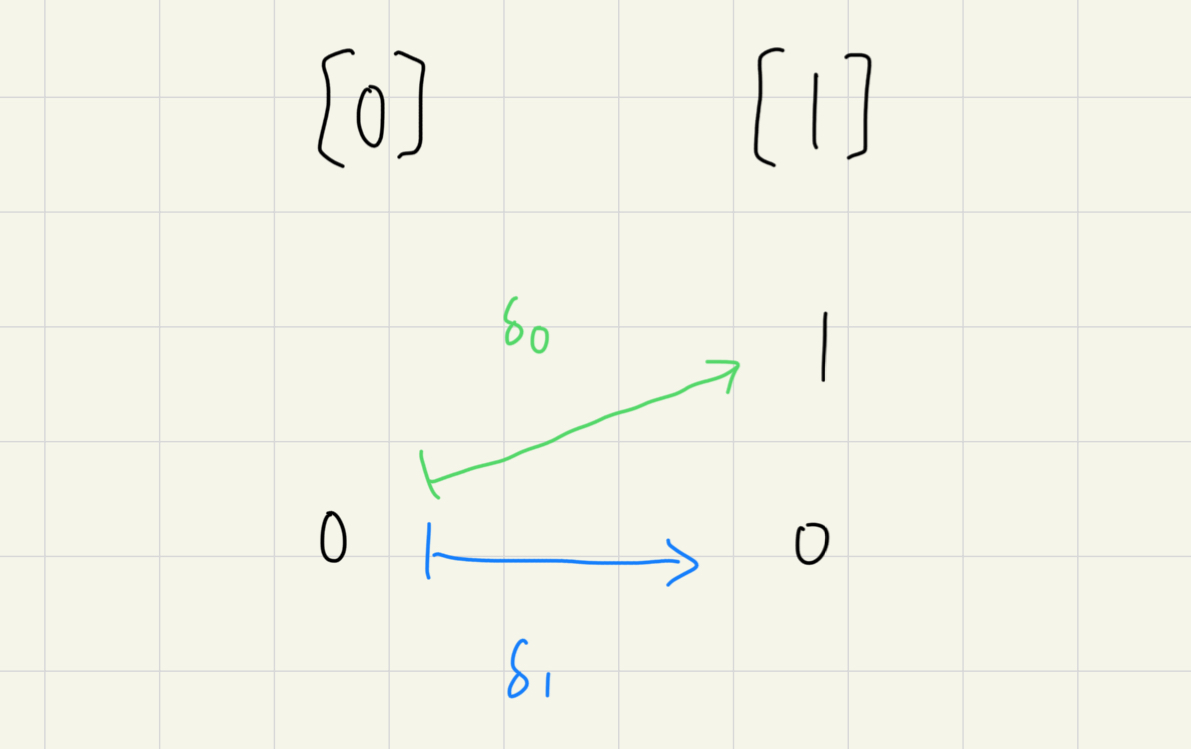
從 到 可以畫成
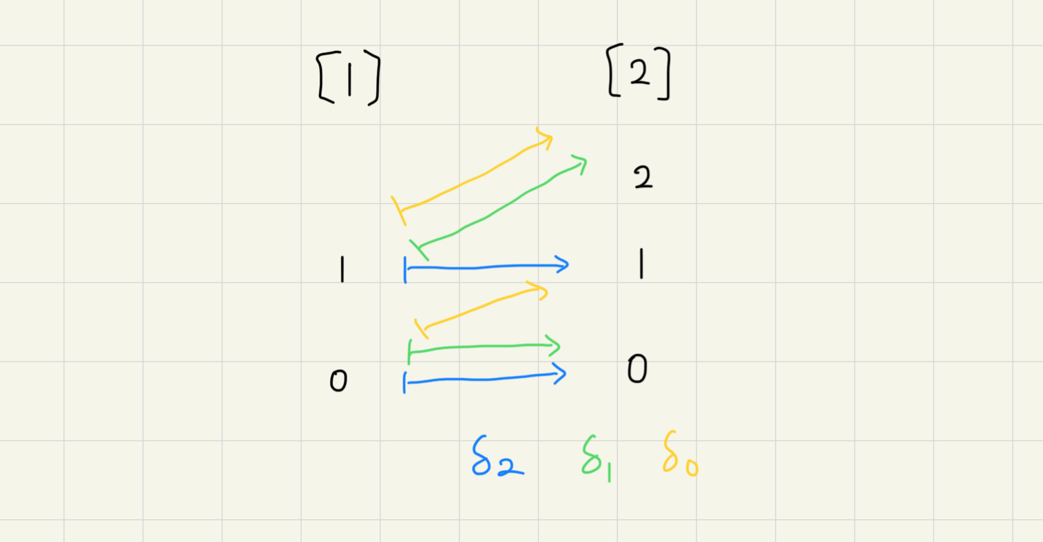
事實上,如果畫成 simplex 的幾何表示 就更明顯了:
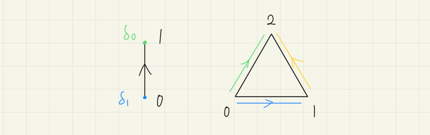
標準 -simplex 可以定義成:
所以 face maps 就是在表示 表示 的哪一個邊界,線的邊界是兩個點,面的邊界是三條線。
沒有內接矩形的平面曲線 [math-001H]
在看過
之後的一點嘗試。
就我的認知,有限多的 singular points 無法破壞這裡的拓墣特性,所以討論非碎形曲線的時候,頂多討論能夠減少內接矩形到什麼程度。所以我真正有興趣的是局部構成沒有內接矩形時,如何重複這個構成還是保持特性。
然而一次跨出這步太超出我目前所知了,所以只能先考慮相關的變形問題:首先,開放的曲線可能沒有內接矩形,比如下圖由兩個有界直線構成(箭頭表示無限延伸方向)
- 如果選擇了頂點與其中一邊的點,那麼法向只能再跟此圖交於一點,無法構成矩形。另一邊因為對稱性所以一樣。
- 如果選擇一邊的兩點,那法向接觸到另一邊的長度不同,自然也不是矩形。
- 如果一邊各自選一點,因為這條邊往任意一邊移動都會改變長度,也沒辦法構成矩形。
但這張圖如果稍作修改,比如加一個直線拉回來變成三角形,就會再次有內接矩形。
另一種值得考慮的基本構造是圓,因為可以說圓的內接矩形有無限多個,但也可以說某種程度上只有一個內接矩形。所以如果考慮取半圓形,另一半則是想辦法破壞對稱性,比如我考慮過的其中一種形狀是
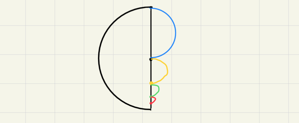
想法就是一直取一半直徑的半圓去填右半部。這個旋轉一下就可以弄成方程組,所以要驗證這個圖形可以嘗試看看方程組中出現矩形要怎麼驗證。
Formal Topology in UF [math-001G]
Reading https://github.com/ayberkt/formal-topology-in-UF and use TypeTopology to understand
Definition Poset [ag-000F]
{-# OPTIONS --safe --without-K #-} module ag-000F where open import MLTT.Spartan open import UF.Sets open import UF.SubtypeClassifier
Order is a binary relation .
order-structure : 𝓤 ̇ → 𝓤 ⁺ ̇ order-structure {𝓤} A = A → A → Ω 𝓤
A poset is a pair
- for all
- and implies for all
- and implies for all
poset-axioms : (A : 𝓤 ̇ ) → order-structure A → 𝓤 ̇ poset-axioms A _≤_ = is-set A × ((x : A) → (x ≤ x) holds) × ((x y z : A) → (x ≤ y) holds → (y ≤ z) holds → (x ≤ z) holds) × ((x y : A) → (x ≤ y) holds → (y ≤ x) holds → x = y) Poset-structure : 𝓤 ̇ → 𝓤 ⁺ ̇ Poset-structure A = Σ _≤_ ꞉ order-structure A , (poset-axioms A _≤_) Poset : (𝓤 : Universe) → 𝓤 ⁺ ̇ Poset 𝓤 = Σ A ꞉ 𝓤 ̇ , Poset-structure A
We can add a helper to extract underlying set
⟨_⟩ : {S : 𝓤 ̇ → 𝓥 ̇ } → Σ S → 𝓤 ̇ ⟨ X , s ⟩ = X order-of : (P : Poset 𝓤) → ⟨ P ⟩ → ⟨ P ⟩ → Ω 𝓤 order-of (X , _≤_ , _) x y = x ≤ y syntax order-of P x y = x ≤⟨ P ⟩ y posets-are-sets : (P : Poset 𝓤) → is-set ⟨ P ⟩ posets-are-sets (X , _≤_ , i , rfl , trans , ir) = i
A hom from a poset to another, is a map that preserves the order
is-hom : (P : Poset 𝓤) (Q : Poset 𝓥) → (⟨ P ⟩ → ⟨ Q ⟩) → 𝓤 ⊔ 𝓥 ̇ is-hom P Q f = ∀ {x y} → (x ≤⟨ P ⟩ y) holds → (f x ≤⟨ Q ⟩ f y) holds
Identity map is a hom
id-is-hom : (P : Poset 𝓤) → is-hom P P id id-is-hom P x≤y = x≤y
The composition of homs is a hom
∘-is-hom : (P : Poset 𝓤) (Q : Poset 𝓥) (R : Poset 𝓦) (f : ⟨ P ⟩ → ⟨ Q ⟩) (g : ⟨ Q ⟩ → ⟨ R ⟩) → is-hom P Q f → is-hom Q R g → is-hom P R (g ∘ f) ∘-is-hom P Q R f g f-is-hom g-is-hom x≤y = g-is-hom (f-is-hom x≤y)
Definition Frame [ag-000G]
{-# OPTIONS --safe --without-K #-} module ag-000G where open import MLTT.Spartan open import UF.SubtypeClassifier open import ag-000F
To build frame, we must be able to talk about arbitrary subsets of underlying set
Fam : 𝓤 ̇ → 𝓤 ⁺ ̇ Fam {𝓤} A = Σ I ꞉ 𝓤 ̇ , (I → A) module JoinSyntax {A : 𝓤 ̇ } (join : Fam A → A) where join-of : {I : 𝓤 ̇ } → (I → A) → A join-of {I} f = join (I , f) syntax join-of (λ i → e) = ∨⟨ i ⟩ e index : {X : 𝓤 ̇ } → Fam X → 𝓤 ̇ index (I , _) = I _$_ : {X : 𝓤 ̇ } → (F : Fam X) → index F → X _$_ (_ , f) = f infixl 40 _$_ _∈_ : {X : 𝓤 ̇ } → X → Fam X → 𝓤 ̇ x ∈ (_ , f) = fiber f x
Beside poset axioms, frame axioms are
- There is a top element , every element
- Binary meet is smaller than and , and it is a limit
- Each arbitrary subset has a join , such that each element of it smaller than the join
- Binary meets must distribute over arbitrary joins
frame-axioms : (X : 𝓤 ̇ ) → order-structure X → X → (X → X → X) → (Fam X → X) → 𝓤 ⁺ ̇ frame-axioms X _≤_ ⊤ _∧_ ∨ = ((x : X) → (x ≤ ⊤) holds) × ((x y : X) → ((x ∧ y) ≤ x) holds × ((x ∧ y) ≤ y) holds) × ((x y z : X) → (z ≤ x) holds → (z ≤ y) holds → (z ≤ (x ∧ y)) holds) × ((U : Fam X) → (x : X) → x ∈ U → (x ≤ ∨ U) holds) × ((U : Fam X) → (x : X) → ((y : X) → y ∈ U → (y ≤ x) holds) → (∨ U ≤ x) holds) × distrib where open JoinSyntax ∨ distrib = ((U : Fam X) → (x : X) → x ∧ (∨ U) = ∨⟨ i ⟩ (x ∧ U $ i)) Frame-structure : 𝓤 ̇ → 𝓤 ⁺ ̇ Frame-structure X = Σ _≤_ ꞉ order-structure X , Σ ⊤ ꞉ X , Σ _∧_ ꞉ (X → X → X) , Σ ∨ ꞉ (Fam X → X) , (poset-axioms X _≤_) × (frame-axioms X _≤_ ⊤ _∧_ ∨) Frame : (𝓤 : Universe) → 𝓤 ⁺ ̇ Frame 𝓤 = Σ X ꞉ 𝓤 ̇ , Frame-structure X
Properties of frames [ag-000H]
{-# OPTIONS --safe --without-K #-} module ag-000H where open import MLTT.Spartan open import UF.SubtypeClassifier open import ag-000F open import ag-000G
In frames, meet is commutative, hence no difference between and
meet-is-comm : (F : Frame 𝓤) → (x y : ⟨ F ⟩) → 𝓤 ̇ meet-is-comm (X , _≤_ , ⊤ , _∧_ , _ ) x y = x ∧ y = y ∧ x prove-meet-is-comm : (F : Frame 𝓤) → (x y : ⟨ F ⟩) → meet-is-comm F x y prove-meet-is-comm (X , _≤_ , ⊤ , _∧_ , ∨ , (_ , _ , _ , split) , (_ , meet , lim , _ , _) ) x y = split (x ∧ y) (y ∧ x) I II where I : ((x ∧ y) ≤ (y ∧ x)) holds I = lim y x (x ∧ y) (meet x y .pr₂) (meet x y .pr₁) II : ((y ∧ x) ≤ (x ∧ y)) holds II = lim x y (y ∧ x) (meet y x .pr₂) (meet y x .pr₁)
Matrix representation of complex numbers [math-001F]
To see why
behave same as the complex numbers is to write as a linear combination:
and hence we are wondering, what if we define
and multiplication as matrix multiplication, addition as matrix addition? Are these behave same as complex numbers? Since is the identity matrix, we simply get followings
we would like to know if :
as desired. Then we also know linear combinations based on and maps to complex numbers bijectively:
so now we can see this indeed is a representation of complex numbers.
旋轉矩陣的 product 是給定角度的相加 [ag-000E]
{-# OPTIONS --without-K #-} module ag-000E where open import MLTT.Spartan hiding (_+_; _×_) open import MLTT.Fin
因為不想引入太多其餘結構,把實數跟三角函數的一些性質直接公理化來用
module _ (ℝ : 𝓤₀ ̇) where variable a b : ℝ postulate cos : ℝ → ℝ sin : ℝ → ℝ -_ : ℝ → ℝ _+_ : ℝ → ℝ → ℝ _×_ : ℝ → ℝ → ℝ tri1 : cos (a + b) = cos a × cos b + - (sin a × sin b) tri2 : sin (a + b) = sin a × cos b + sin b × cos a ℝ-neg-1 : a × - b = - (a × b) ℝ-neg-add : - a + - b = - (a + b) ℝ-+-comm : a + b = b + a ℝ-×-comm : a × b = b × a infixl 60 -_ infixl 40 _+_ infixl 50 _×_ ℝ-neg-2 : - a × b = - (a × b) ℝ-neg-2 {a}{b} = - a × b =⟨ ℝ-×-comm ⟩ b × - a =⟨ ℝ-neg-1 ⟩ - (b × a) =⟨ ap -_ ℝ-×-comm ⟩ - (a × b) ∎
矩陣可以看成由兩個索引指向某其 Field 的元素的型別
Matrix : (m n : ℕ) → (K : 𝓤 ̇) → 𝓤 ̇ Matrix m n K = Fin m → Fin n → K
只定義 的矩陣乘法
_⊗_ : Matrix 2 2 ℝ → Matrix 2 2 ℝ → Matrix 2 2 ℝ _⊗_ m n 𝟎 𝟎 = m 𝟎 𝟎 × n 𝟎 𝟎 + m 𝟎 𝟏 × n 𝟏 𝟎 _⊗_ m n 𝟎 𝟏 = m 𝟎 𝟎 × n 𝟎 𝟏 + m 𝟎 𝟏 × n 𝟏 𝟏 _⊗_ m n 𝟏 𝟎 = m 𝟏 𝟎 × n 𝟎 𝟎 + m 𝟏 𝟏 × n 𝟏 𝟎 _⊗_ m n 𝟏 𝟏 = m 𝟏 𝟎 × n 𝟎 𝟏 + m 𝟏 𝟏 × n 𝟏 𝟏 infixl 30 _⊗_
旋轉矩陣它本人,這個用來表示 ,其中 是角度的值
R : ℝ → Matrix 2 2 ℝ R θ 𝟎 𝟎 = cos θ R θ 𝟎 𝟏 = sin θ R θ 𝟏 𝟎 = - sin θ R θ 𝟏 𝟏 = cos θ
證明目標:
證明方式就是按 component 去證明等式成立。
thm : {θ φ : ℝ} (i j : Fin 2) → (R θ ⊗ R φ) i j = R (θ + φ) i j thm {θ}{φ} 𝟎 𝟎 = (R θ ⊗ R φ) 𝟎 𝟎 =⟨by-definition⟩ cos θ × cos φ + sin θ × (- sin φ) =⟨ ap (cos θ × cos φ +_) ℝ-neg-1 ⟩ cos θ × cos φ + - (sin θ × sin φ) =⟨ tri1 ⁻¹ ⟩ cos (θ + φ) =⟨by-definition⟩ R (θ + φ) 𝟎 𝟎 ∎ thm {θ}{φ} 𝟎 𝟏 = (R θ ⊗ R φ) 𝟎 𝟏 =⟨by-definition⟩ cos θ × sin φ + sin θ × cos φ =⟨ ℝ-+-comm ⟩ sin θ × cos φ + cos θ × sin φ =⟨ ap (sin θ × cos φ +_) ℝ-×-comm ⟩ sin θ × cos φ + sin φ × cos θ =⟨ tri2 ⁻¹ ⟩ sin (θ + φ) =⟨by-definition⟩ R (θ + φ) 𝟎 𝟏 ∎ thm {θ}{φ} 𝟏 𝟎 = (R θ ⊗ R φ) 𝟏 𝟎 =⟨by-definition⟩ (- sin θ) × cos φ + cos θ × (- sin φ) =⟨ ap (_+ cos θ × - sin φ) ℝ-neg-2 ⟩ - (sin θ × cos φ) + cos θ × (- sin φ) =⟨ ap (- (sin θ × cos φ) +_) ℝ-neg-1 ⟩ - (sin θ × cos φ) + - (cos θ × sin φ) =⟨ ℝ-neg-add ⟩ - (sin θ × cos φ + cos θ × sin φ) =⟨ ap -_ (ap (sin θ × cos φ +_) ℝ-×-comm) ⟩ - (sin θ × cos φ + sin φ × cos θ) =⟨ ap -_ (tri2 ⁻¹) ⟩ - sin (θ + φ) =⟨by-definition⟩ R (θ + φ) 𝟏 𝟎 ∎ thm {θ}{φ} 𝟏 𝟏 = (R θ ⊗ R φ) 𝟏 𝟏 =⟨by-definition⟩ - sin θ × sin φ + cos θ × cos φ =⟨ ℝ-+-comm ⟩ cos θ × cos φ + - sin θ × sin φ =⟨ ap (cos θ × cos φ +_) ℝ-neg-2 ⟩ cos θ × cos φ + - (sin θ × sin φ) =⟨ tri1 ⁻¹ ⟩ R (θ + φ) 𝟏 𝟏 ∎ addition : {θ φ : ℝ} (i j : Fin 2) → (R θ ⊗ R φ) i j = (R φ ⊗ R θ) i j addition {θ} {φ} i j = (R θ ⊗ R φ) i j =⟨ thm i j ⟩ R (θ + φ) i j =⟨ ap (λ x → R x i j) ℝ-+-comm ⟩ R (φ + θ) i j =⟨ thm i j ⁻¹ ⟩ (R φ ⊗ R θ) i j ∎
Streams and finite observations [ag-000D]
From Topology via logic
{-# OPTIONS --safe --without-K --guardedness --no-exact-split #-} module ag-000D where open import MLTT.Spartan open import MLTT.List
Stream can be defined as a coinductive record.
record Stream (A : 𝓤 ̇ ) : 𝓤 ̇ where coinductive constructor _∷_ field head : A tail : Stream A open Stream
For example a stream of all zero.
zeros : Stream 𝟚 head zeros = ₀ tail zeros = zeros
s ⊨starts o defines a relation that a stream can be
realized by a finite observation.
_⊨starts_ : Stream 𝟚 → List 𝟚 → 𝓤₀ ̇ s ⊨starts [] = ₀ = ₀ s ⊨starts (x ∷ xs) = (x = head s) × (tail s ⊨starts xs)
For example, the first bit zeros produces is
₀.
first-bit : zeros ⊨starts [ ₀ ] first-bit = refl , refl
Every stream can be realized by “no” observation.
realize-by-no-observation : (s : Stream 𝟚) → s ⊨starts [] realize-by-no-observation s = refl
We can define order relation for these finite observations.
_⊇_ : List 𝟚 → List 𝟚 → 𝓤₀ ̇ _ ⊇ [] = ₀ = ₀ [] ⊇ _ = 𝟘 (x ∷ l) ⊇ (x₁ ∷ l2) = (x = x₁) × (l ⊇ l2)
This order has antisymmetric
eq-condition : (l1 l2 : List 𝟚) → l1 ⊇ l2 → l2 ⊇ l1 → l1 = l2 eq-condition [] [] p q = refl eq-condition (x ∷ l1) (y ∷ l2) (ph , pt) (qh , qt) = x ∷ l1 =⟨ ap (_∷ l1) ph ⟩ y ∷ l1 =⟨ ap (y ∷_) (eq-condition l1 l2 pt qt) ⟩ y ∷ l2 ∎
, in fact total, which means a boring order. The order induces refinement of observations: if a observation is subsequence of another observation that realise the stream, then the stream also be realized by this subsequence.
refine-observation : {s : Stream 𝟚} → (l l2 : List 𝟚) → s ⊨starts l → l ⊇ l2 → s ⊨starts l2 refine-observation l2 [] _ _ = refl refine-observation (x ∷ l) (y ∷ l2) (x=head , tail) (x=y , rest) = (x=y ⁻¹ ∙ x=head) , refine-observation l l2 tail rest
Dependent equality in dependent type theory [ag-000C]
這是從 https://mathstodon.xyz/@MartinEscardo/114751426538568913 學到的技巧。
{-# OPTIONS --safe --without-K #-} module ag-000C where open import Agda.Primitive renaming (Set to Type; Setω to Typeω) open import Agda.Builtin.Equality open import Agda.Builtin.Nat
假設我們有
- a type
X : Type - a family of types
A : X → Typeindexed byX
那我們常常會遇到有
x y : Xa : A xb : A yp : x = y
= 是 MLTT 的 identity type,p 是一個
x = y 的證明,這時候如果我們問 a = b
是沒有答案的,因為根據 MLTT,a 跟 b
的類型壓根兒就不一樣,這導致問題連寫都寫不下來,那怎麼辦?
方法是定義高階等式(又稱為 dependent equality 或是 PathOver 或是 path transport),在該依賴項等價的情況下把問題變成新的等式來讓 dependent type 語言表達等式
用案例來說就是如果有個 equality 是「類型不同」的(出於依賴項的不透明性,比如這裡 vector length 輸入的 associative 不同)
先定義一些下面案例會用到的輔助程式:
cong : {X Y : Type} (f : X → Y) {x₀ x₁ : X} → x₀ ≡ x₁ → f x₀ ≡ f x₁ cong {X} {Y} f refl = refl +-assoc : ∀ l m n → (l + m) + n ≡ l + (m + n) +-assoc zero m n = refl +-assoc (suc l) m n = cong suc (+-assoc l m n)
具體案例 vector ++ 的 associativity
data Vec (A : Type) : Nat → Type where [] : Vec A 0 _::_ : ∀{n} → A → Vec A n → Vec A (suc n) infixl 40 _::_ _++_ : {Y : Type} {l m : Nat} → (xs : Vec Y l) → (ys : Vec Y m) → Vec Y (l + m) [] ++ ys = ys (x :: xs) ++ ys = x :: (xs ++ ys) infixl 30 _++_
基於 x₀ ≡ x₁ 定義一個更高階的 equality
higher-equality : {X : Type} (A : X → Type) {x₀ x₁ : X} → A x₀ → x₀ ≡ x₁ → A x₁ → Type higher-equality A a₀ refl a₁ = a₀ ≡ a₁
但可以根據案例定義比較簡單的版本
_≡[_]_ : {X : Type} {x₀ x₁ : Nat} → Vec X x₀ → x₀ ≡ x₁ → Vec X x₁ → Type a₀ ≡[ refl ] a₁ = a₀ ≡ a₁
命題 (xs ++ ys) ++ zs ≡ xs ++ (ys ++ zs)
無法寫下,因為(meta-level 的)型別不同。 所以需要用高階等式描述
cong-cons : {X : Type} {m n : Nat} {xs : Vec X m} {ys : Vec X n} (x : X) (p : m ≡ n) → xs ≡[ p ] ys → x :: xs ≡[ cong suc p ] x :: ys cong-cons {X}{A} x refl refl = refl ++-assoc : {X : Type} (l m n : Nat) (xs : Vec X l) (ys : Vec X m) (zs : Vec X n) → (xs ++ ys) ++ zs ≡[ +-assoc l m n ] xs ++ (ys ++ zs) ++-assoc {X} zero m n [] ys zs = refl ++-assoc {X} (suc l) m n (x :: xs) ys zs = I where I : x :: (xs ++ ys) ++ zs ≡[ cong suc (+-assoc l m n) ] x :: (xs ++ (ys ++ zs)) I = cong-cons x (+-assoc l m n) (++-assoc l m n xs ys zs)
Second-Order Generalised Algebraic Theories: Signatures and First-Order Semantics [tt-000U]
NOTE about Second-Order Generalised Algebraic Theories: Signatures and First-Order Semantics
這篇文章主要在探討程式語法的表示方式,並展示如何結合代數方法跟 HOAS。作者說他們跟隨 Uemura 把語言定義成 second-order generalised algebraic theories (SOGATs),通過一系列案例揭示 non-substructural languages 可以自然的定義成 SOGATs
- SOGAT 的形式定義 (using the syntax of a particular SOGAT)
- 定義兩種 SOGAT signatures 到 GAT signatures (signatures for quotient inductive-inductive types) 的轉換,分別基於同時替換(parallel substitution)與單一替換(single substitution)
按代數抽象程度區分 [local-0]
從具體到抽象可以把語法表示看成
| 語法表示 | 能力 |
| abstract syntax trees (AST) | 把程式原文 parse 後直接儲存用的一系列資料結構 |
| well-scoped syntax tree | λx.x 跟 λy.y 在這類表示法裡面無法區分,也就是說綁定使用的具體名稱不再重要 |
| intrinsic well-typed terms | 這種表示把語法跟 typing relation 整合,所以 non well-typed 的程式甚至無法表達 |
| well-typed, quotiented by the conversion relation (GAT) | 加上更多 well-formness relation 的推廣代數理論,下面介紹 |
| SOGAT | GAT 推到 second-order,下面介紹 |
在 well-typed terms 上再加上 conversion relation 就變成廣義代數理論(generalised algebraic theory,簡稱 GAT),GAT 用來處理 dependently typed languages 時特別方便,因為 typing 依賴了 conversion relation。在 GAT 上只能定義保留了 conversion relation 的函數,因此連印出函數都無法定義,但 normalisation(正規化)、typechecking(型別檢查)跟 parametricity 這些函數保留 conversion 因此可定義。
對任何 GAT 來說,syntax 可以定義成 initial model,因此沒有區分語法跟語意的必要,某種意義上來說,一個程式語言就是一個 GAT。
HOAS 方法:按對 bindings/variables 的處理方式區分 [local-1]
HOAS 觀點關心 bindings 跟 variables 的處理方式,比如 De Bruijn indices 使名稱選擇與語意無關,但這也表示替換必須是語法的一部分,舉例來說 form of a category with families。
Logical frameworks 跟 higher-order abstract syntax (HOAS) 提供了另一種實現 bindings 跟 variables 的方式:使用 metatheory 的函數空間。
舉例來說,pure lambda calculus 的 lambda operation 的 type 是二階函數空間 (Tm → Tm) → Tm。這在理論上的解釋是 type-theoretic internal language of presheaves over the category of contexts and syntactic substitutions,在這個 topos 的 internal language 裡,lambda 的類型就長那樣。
Internal language 的觀點可以用來定義程式語言是什麼:有綁定的語言不是一個 GAT,而是一個二階的廣義代數理論(second-order generalised algebraic theory,簡稱 SOGAT),這種理論可以有二階操作(但不是任意高階)。
Untyped 或是 Simply typed 都有被定義成二階理論過,但 Uemura 是第一個用 SOGATs 定義有綁定的語言的人。這個理論真的很厲害,一個語言的 SOGAT 定義比 well-typed quotiented 定義還要抽象:SOGAT 連 contexts 跟 substitutions 都不用提到,這些會自動生成。但這不是一個 well-behaved 的代數理論,比如 second-order models 之間沒有有意義的 homomorphism。
為了描述 SOGAT 的一階模型、homomorphisms 或是 syntax 的 notion,作者把它轉成一個 GAT。這個過程中引入新的 sorts 給 contexts 跟 substitutions,然後把每個操作都用其 context index,second-order 的函數空間也由 context indexing 轉換成 first-order。因此得到一個有 some “correctness by construction” properties 的 GAT,比如每個操作都自動保留替換。這對複雜的理論來說,如果不是從 SOGAT 出發而是直接用其 GAT 表示,那這種屬性並不 trivial。
Cubical type theory 跟有 internal parametricity 的 type theory 都可以定義成 SOGATs,這些方法已經用來證明型別論的屬性。
Substructural (像是 linear or modal) type theories 無法用這篇論文說的方法用 SOGATs 定義,但有時候 presheaves over a substructural theory 提供的 substructural internal language 可以用來描述理論,像是 multi-modal type theory。
簡單的代數理論可以用 signatures 和方程式來表示,也可以 presentation independently 為 Lawvere theories。
GATs 的 syntactic signatures 可以用 preterms 跟 well-formedness relations 定義,也可以 presentation-independent 為 contextual categories 或 categories with families (CwFs) 或 clans。
GATs 的 theory of signatures (ToS) 方法落在 syntactic 跟 presentation-independent 方法中間:signatures 用某個 GAT 語法定義,這是一種設計來專用於定義簽名的類型理論。簽名跟我們在 Agda 裡寫下的 inductive datatype 定義一模一樣:A list (telescope) of the curried types of sorts and constructors。ToS 裡一個 signature 是一個理論的具體表示,但在 well-typed quotiented syntax 這層抽象上給出。這讓我們得到優雅的語意構造,又還是能用 signatures 工作。
SOGATs 同樣可以定義成 syntactically 或 presentation-independently(用 representable map categories 或是 CwFs with locally representable types)
這篇論文貢獻了 ToS 風格的 SOGATs 定義。SOGAT signatures 的理論本身也是 SOGAT,所以這個理論可以描述自己。
避免了循環論證,因為我們首先將 SOGAT 簽名定義為 GAT,從而引導 SOGAT 簽名理論,而 GAT 簽名理論(即 GAT 的語法)本身可以使用 Church 編碼進行引導。
Contributions [local-2]
The main takeaway of this paper is that structural languages are SOGATs.
We justify this claim through several examples. Our technical contributions are the following:
- The theory of SOGAT signatures (ToS+), a domain-specific type theory in which every closed type is a SOGAT signature. As it is a structural type theory, it can be defined as a SOGAT itself. Signatures can be formalised in ToS+ without encoding overhead.
- A translation from SOGAT signatures to GAT signatures based on a parallel substitution calculus. Thus, for every SOGAT, we obtain all of the semantics of GATs: a category of models with an initial object, (co)free models, notions of displayed models and sections, the fact that induction is equivalent to initiality, and so on. The GAT descriptions that we obtain are readable, do not contain occurrences of Yoneda as in usual presheaf function spaces. Correctness of the translation is showed by proving that internally to presheaves over a model of the GAT, a second-order model of the SOGAT is available.
- We define an alternative translation producing a single substitution calculus.
作者開始展示如何把各種 logic 或程式語言定義成代數理論。這邊我寫下每個代數理論的 agda 版本
Schönfinkel's combinator calculus (Algebraic Theories) [ag-0003]
{-# OPTIONS --safe --without-K #-} module ag-0003 where open import MLTT.Spartan
Combinator calculus 可以看成一個代數理論,這時候它有
- 一個 sort of terms
- 一個 binary
- 兩個 nullary operations
- 兩個等式
record combinator-calculus : 𝓤₁ ̇ where field Tm : 𝓤₀ ̇ _·_ : Tm → Tm → Tm K : Tm S : Tm Kβ : {u f : Tm} → K · u · f = u Sβ : {f g u : Tm} → S · f · g · u = f · u · (g · u) infixl 30 _·_
- 從這個符號可以明顯看出代數/模型的概念
- Combinator calculus 的 quotiented syntax 是初始模型,它總是存在。
- Notions of homomorphism, displayed/dependent model, induction, products and coproducts of models, free models, and so on, are derivable from the signature, as described in any book on universal algebra
- Algebraic Theory 的 initial algebra 叫做 quotient inductive type
其他 single-sorted algebraic theories 著名案例:
- 邏輯:經典(或直覺主義)命題邏輯,定義為布林代數(或海廷代數)理論
- 代數:monoids、群、環、lattices 等等
Generalised algebraic theories (GATs) [local-3]
Generalised algebraic theories (GATs) 的 sort 可以 indexed by 其他 sort。案例有 typed combinator calculus、propositional logic with Hilbert-style proof theory、theories of graphs、preorders、categories 等等
Typed combinator calculus (Generalised algebraic theories) [ag-0004]
{-# OPTIONS --safe --without-K #-} module ag-0004 where open import MLTT.Spartan
record typed-combinator-calculus : 𝓤₁ ̇ where field
給 types 的 sort
Ty : 𝓤₀ ̇
每個 type 對應(index)一個 term 用的 sort
Tm : Ty → 𝓤₀ ̇ ι : Ty _⇒_ : Ty → Ty → Ty _·_ : {A B : Ty} → Tm (A ⇒ B) → Tm A → Tm B K : {A B : Ty} → Tm (A ⇒ B ⇒ A) S : {A B C : Ty} → Tm ((A ⇒ B ⇒ C) ⇒ (A ⇒ B) ⇒ A ⇒ C) Kβ : {A B : Ty} {u : Tm A} {f : Tm B} → K · u · f = u Sβ : {A B C : Ty} {f : Tm (A ⇒ B ⇒ C)} {g : Tm (A ⇒ B)} {u : Tm A} → S · f · g · u = f · u · (g · u) infixl 40 _·_ infixr 30 _⇒_
上述 Algebraic Theory 的通用代數特徵可以推廣到 GAT。具體來說,每個 GAT 都具有由 quotient inductive-inductive type 給出的語法,我們有 free 模型和 cofree 模型。
Second-order algebraic theories (SOATs) [local-4]
如果一個語言有變數或是綁定,就被定義成一個二階理論。
Lambda calculus (Second-order algebraic theories) [ag-0005]
{-# OPTIONS --safe --without-K #-} module ag-0005 where open import MLTT.Spartan
record lambda-calculus : 𝓤₁ ̇ where field Tm : 𝓤₀ ̇
lam 的(metatheory)型別不是一階的(not strictly
positive)
lam : (Tm → Tm) → Tm _·_ : Tm → Tm → Tm β : {f : Tm → Tm} {u : Tm} → lam f · u = f u infixl 30 _·_
By the syntax of lambda calculus, we mean the syntax for the GAT of Definition 4. However, we still prefer to define lambda calculus as a SOGAT: it is a shorter definition, does not include boilerplate, and ensures that once translated to its first-order version, all operations respect substitution by construction.
此外,我們可以像邏輯框架一樣,使用二階表示來進行程式設計。這意味著,使用二階表示,我們可以定義 derivable operation 並證明 derivable 等式,而不是像證明 admissible 那樣需要歸納法。
舉例來說 Y combinator 是 derivable operation。可以證明它是 fixpoint combinator:
Y : Tm Y = lam (λ f → (lam (λ x → f · (x · x))) · (lam (λ x → f · (x · x)))) Y-is-fixed-point : {f : Tm} → Y · f = f · (Y · f) Y-is-fixed-point {f} = Y · f =⟨by-definition⟩ lam (λ f → (lam (λ x → f · (x · x))) · (lam (λ x → f · (x · x)))) · f =⟨ β ⟩ (λ f → (lam (λ x → f · (x · x))) · (lam (λ x → f · (x · x)))) f =⟨ refl ⟩ (lam (λ x → f · (x · x))) · (lam (λ x → f · (x · x))) =⟨ β ⟩ f · ((lam (λ x → f · (x · x))) · (lam (λ x → f · (x · x)))) =⟨ refl ⟩ f · ((λ f → (lam (λ x → f · (x · x))) · (lam (λ x → f · (x · x)))) f) =⟨ ap (f ·_) (β ⁻¹) ⟩ f · (Y · f) ∎
這種推理對任何 second-order model 都有效,而且任何 first-order model 都可以在 internal language of presheaves over first-order model 裡被升級成 second-order model。
但注意沒有可用的 SOAT models 和 之間的同態概念。為了討論同態或語法,我們將 SOAT 轉換為一階 GAT:加上上下文、替換、索引 Tm 以及所有基於上下文的操作,然後 lam 就變成了一個以擴展上下文中的項作為輸入的一階函數。轉換出來的 GAT 就是
Lambda calculus (GAT) [ag-0006]
{-# OPTIONS --safe --without-K #-} module ag-0006 where open import MLTT.Spartan hiding (_∘_; id)
作者這邊開始解釋從二階理論得出一階理論(GAT)的標準過程
record first-order-lambda-calculus : 𝓤₁ ̇ where field Con : 𝓤₀ ̇ Sub : Con → Con → 𝓤₀ ̇
有 terminal object 的 category
_∘_ : {Δ Γ Θ : Con} → Sub Δ Γ → Sub Θ Δ → Sub Θ Γ assoc : {A B C D : Con} {γ : Sub C D} {δ : Sub B C} {θ : Sub A B} → (γ ∘ δ) ∘ θ = γ ∘ (δ ∘ θ) id : {Γ : Con} → Sub Γ Γ id-left : {A B : Con} {γ : Sub A B} → id ∘ γ = γ id-right : {A B : Con} {γ : Sub A B} → γ ∘ id = γ -- empty context: zero ◇ : Con ε : {Γ : Con} → Sub Γ ◇ -- terminal ◇η : {Γ : Con} → (σ : Sub Γ ◇) → σ = ε
sort Tm 現在 indexed by Con 且有一個
instantiation operation,這個 operation 是 functorial
([◦], [id]).
Tm : Con → 𝓤₀ ̇ _[_] : {Γ Δ : Con} → Tm Γ → Sub Δ Γ → Tm Δ [id] : {Γ : Con} {t : Tm Γ} → t [ id ] = t [∘] : {Θ Γ Δ : Con} {t : Tm Γ} {γ : Sub Δ Γ} {δ : Sub Θ Δ} → t [ γ ∘ δ ] = t [ γ ] [ δ ]
context extension 讓 contexts 是 natural number algebra
_▹ : Con → Con
substitutions 是一串 terms,由組成元件表達
_,,_ : {Δ Γ : Con} → Sub Δ Γ → Tm Δ → Sub Δ (Γ ▹)
有了 contexts 跟 substitutions,變數就可以定義成 De Bruijn indices:
0 = q1 = q[p]2 = q[p] [p],以此類推
p : {Γ : Con} → Sub (Γ ▹) Γ q : {Γ : Con} → Tm (Γ ▹)
應該滿足的等式規則
▹β₁ : {Δ Γ : Con} {γ : Sub Δ Γ} {t : Tm Δ} → p ∘ (γ ,, t) = γ ▹β₂ : {Δ Γ : Con} {γ : Sub Δ Γ} {t : Tm Δ} → q [ γ ,, t ] = t ▹η : {Δ Γ : Con} {σ : Sub Δ (Γ ▹)} → σ = (p ∘ σ ,, q [ σ ]) lam : {Γ : Con} → Tm (Γ ▹) → Tm Γ lam[] : {Δ Γ : Con} {γ : Sub Δ Γ} {t : Tm (Γ ▹)} → (lam t)[ γ ] = lam (t [ γ ∘ p ,, q ]) _·_ : {Γ : Con} → Tm Γ → Tm Γ → Tm Γ ·[] : {Δ Γ : Con} {γ : Sub Δ Γ} {t u : Tm Γ} → (t · u)[ γ ] = t [ γ ] · (u [ γ ]) β : {Δ Γ : Con} {γ : Sub Δ Γ} {t : Tm (Γ ▹)} {u : Tm Γ} → lam t · u = t [ id ,, u ] infixl 40 _∘_ infixl 30 _,,_ infixl 40 _·_ infixl 50 _[_]
Second-order generalised algebraic theories (SOGATs) [local-5]
SOGATs combine the two previous classes: sorts can be indexed over previous sorts and second-order operations are allowed.
Simply typed lambda calculus [ag-0007]
{-# OPTIONS --safe --without-K #-} module ag-0007 where open import MLTT.Spartan open import UF.Equiv
record simply-typed-lambda-calculus : 𝓤₁ ̇ where field Ty : 𝓤₀ ̇ _⇒_ : Ty → Ty → Ty
generalised 的部分是因為 index Tm by Ty
Tm : Ty → 𝓤₀ ̇
綁定的部分
lam : {A B : Ty} → (Tm A → Tm B) → Tm (A ⇒ B) _·_ : {A B : Ty} → Tm (A ⇒ B) → (Tm A → Tm B) stlc-cong : {A B : Ty} → Tm (A ⇒ B) ≃ (Tm A → Tm B)
一樣參照 first-order lambda calculus 的過程,加上 contexts、加上 substitutions,相應的 first-order 等式跟改寫,就會得到 simply-typed-lambda-calculus 的 GAT。
Minimal intuitionistic first-order logic (SOGAT) [ag-0008]
{-# OPTIONS --safe --without-K #-} module ag-0008 where open import MLTT.Spartan open import UF.Subsingletons
record minimal-intuitionistic-first-order-logic : 𝓤₁ ̇ where field For : 𝓤₀ ̇ Tm : 𝓤₀ ̇ _⊃_ : For → For → For All : (Tm → For) → For Eq : Tm → Tm → For Pf : For → 𝓤₀ ̇ Pf-is-prop : (A : For) → is-prop (Pf A) intro⊃ : {A B : For} → (Pf A → Pf B) → Pf (A ⊃ B) elim⊃ : {A B : For} → Pf (A ⊃ B) → (Pf A → Pf B) intro∀ : {A : Tm → For} → ((𝑡 : Tm) → Pf (A 𝑡)) → Pf (All A) elim∀ : {A : Tm → For} → Pf (All A) → ((𝑡 : Tm) → Pf (A 𝑡)) introEq : {t : Tm} → Pf (Eq t t) elimEq : {t t' : Tm} → (A : Tm → For) → Pf (Eq t t') → Pf (A t) → Pf (A t')
一樣參照 first-order lambda calculus 的過程,加上 contexts、加上 substitutions,相應的 first-order 等式跟改寫。
Polymorphic lambda calculus (SOGAT) [ag-0009]
{-# OPTIONS --safe --without-K #-} module ag-0009 where open import MLTT.Spartan
record polymorphic-lambda-calculus : 𝓤₁ ̇ where field Ty : 𝓤₀ ̇ Tm : Ty → 𝓤₀ ̇ _⇒_ : Ty → Ty → Ty lam : {𝐴 𝐵 : Ty} → (Tm 𝐴 → Tm 𝐵) → Tm (𝐴 ⇒ 𝐵) _·_ : {𝐴 𝐵 : Ty} → Tm (𝐴 ⇒ 𝐵) → (Tm 𝐴 → Tm 𝐵) All : (Ty → Ty) → Ty Lam : {𝐴 : Ty → Ty} → ((𝑋 : Ty) → Tm (𝐴 𝑋)) → Tm (All 𝐴) _•_ : {𝐴 : Ty → Ty} → Tm (All 𝐴) → ((𝑋 : Ty) → Tm (𝐴 𝑋))
一樣參照 first-order lambda calculus 的過程,加上 contexts、加上 substitutions,相應的 first-order 等式跟改寫。
System Fω (SOGAT) [ag-000A]
{-# OPTIONS --safe --without-K #-} module ag-000A where open import MLTT.Spartan
record system-F-ω : 𝓤₁ ̇ where field □ : 𝓤₀ ̇ Ty : □ → 𝓤₀ ̇ _⇛_ : □ → □ → □ LAM : {K L : □} → (Ty K → Ty L) → Ty (K ⇛ L) _●_ : {K L : □} → Ty (K ⇛ L) → (Ty K → Ty L) ∗ : □ Tm : Ty ∗ → 𝓤₀ ̇ All : {K : □} → (Ty K → Ty ∗) → Ty ∗ Lam : {K : □}{A : Ty K → Ty ∗} → ((X : Ty K) → Tm (A X)) → Tm (All A) _•_ : {K : □}{A : Ty K → Ty ∗} → Tm (All A) → ((X : Ty K) → Tm (A X)) _⇒_ : Ty ∗ → Ty ∗ → Ty ∗ lam : {A B : Ty ∗} → (Tm A → Tm B) → Tm (A ⇒ B) _·_ : {A B : Ty ∗} → Tm (A ⇒ B) → (Tm A → Tm B)
System Fω 轉換後有
- 3 個 operations 綁定 Ty-variables
- 1 個 operation 綁定 term-variable
Minimal Martin-Löf type theory (SOGAT) [ag-000B]
{-# OPTIONS --safe --without-K #-} module ag-000B where open import MLTT.Spartan open import MLTT.NaturalNumbers
variable 𝑖 : ℕ record minimal-martin-lof-type-theory : 𝓤₁ ̇ where field Ty : ℕ → 𝓤₀ ̇ U : (𝑖 : ℕ) → Ty (succ 𝑖) Tm : Ty 𝑖 → 𝓤₀ ̇ c : Ty 𝑖 → Tm (U 𝑖) El : Tm (U 𝑖) → Ty 𝑖 PI : (A : Ty 𝑖) → (Tm A → Ty 𝑖) → Ty 𝑖 Lift : Ty 𝑖 → Ty (succ 𝑖) lam : {𝐴 : Ty 𝑖}{𝐵 : Tm 𝐴 → Ty 𝑖} → ((𝑎 : Tm 𝐴) → Tm (𝐵 𝑎)) → Tm (PI 𝐴 𝐵) _·_ : {𝐴 : Ty 𝑖}{𝐵 : Tm 𝐴 → Ty 𝑖} → Tm (PI 𝐴 𝐵) → ((𝑎 : Tm 𝐴) → Tm (𝐵 𝑎)) mk : {𝐴 : Ty 𝑖} → Tm 𝐴 → Tm (Lift 𝐴) un : {𝐴 : Ty 𝑖} → Tm (Lift 𝐴) → Tm 𝐴
這個理論的對應 GAT
得到一個具有族的範疇(CwF),更準確地說,是一個具有 N 個 families
的範疇,這些族配備了 familywise Π-types、宇宙以及族之間的一步向上提升。
這些類型是 Ty : Con → N → Set 和
Tm : (Γ : Con) → Ty Γ 𝑖 → Set,其中 𝑖
論證隱含在後者中。
後面幾節
- 第三節 Theories of signatures as SOGATs,開始把 signatures 理論也寫成 SOGAT 來討論
- 第四節 Naive semantics of SOGAT signatures,討論 for any SOGAT signature 的 a notion of first-order model.
- 第五節 Direct semantics of SOGAT signatures,用一個更小心版本的 presheaf model 定義 first-order models of SOGATs
- 第六節 GAT signature semantics of SOGAT signatures,把 SOGAT signatures 轉成 GAT signatures 的方法
Intrinsically typed term [ag-0002]
{-# OPTIONS --safe --without-K #-} module ag-0002 where open import MLTT.Spartan hiding (Type) open import MLTT.List
Type 在 STLC 還只需要是一個簡單的 formation
data Type : 𝓤₀ ̇ where bool : Type _⇒_ : Type → Type → Type infixr 50 _⇒_ variable S T : Type
Context 通常會自訂,比如 MLTT 需要兩種綁定時自訂就會更方便一些
Ctx = List Type _▷_ : Ctx → Type → Ctx Γ ▷ T = T ∷ Γ infix 40 _▷_ variable Γ : Ctx
Intrinsically-scoped de Brujin indices
基本上變數都長這樣
data _∋_ : Ctx → Type → 𝓤₀ ̇ where here : Γ ▷ T ∋ T there : Γ ∋ T → Γ ▷ S ∋ T infix 20 _∋_ variable x : Γ ∋ T
Intrinsically-typed terms
確保 term 是類型良好的一種方式就是從一開始就跟 context 一起構造,讓 terms 必須是 well-typed
data _⊢_ : Ctx → Type → 𝓤₀ ̇ where true false : Γ ⊢ bool var : Γ ∋ T → Γ ⊢ T lam : Γ ▷ S ⊢ T → Γ ⊢ S ⇒ T _·_ : Γ ⊢ S ⇒ T → Γ ⊢ S → Γ ⊢ T if_then_else_ : Γ ⊢ bool → Γ ⊢ T → Γ ⊢ T → Γ ⊢ T infix 30 _⊢_
Video Why You Can't Bring Checkerboards to Math Exams [math-001E]
A cool way to do multiply, divide and root!
Definition Diffeological space [math-001D]
A diffeological space is a pair consists of a given set and a diffeology consists of a collection of parameterizations satisfying the following conditions:
- All parameterizations with domain belong to , namely all the points of
- If is a parameterization, and is a smooth map between cartesian spaces, then belongs to
- If is a parameterization, an open cover of that each restriction , then
If is a diffeology, then we call a parameterization that belongs to it a plot.
Lemma Presheaves are colimits of representables [math-001B]
The presheaf is the colimit of the functor ,
where is the yoneda embedding, is the category of elements of . For morphism .
Proof [local-0]
We first show that is a cocone, for each object , there is a morphism
here abuse notation that has a corresponding in because the Yoneda lemma.
and for each , the following diagram commutes
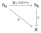
hence is a cocone. Given any other cocone , which means a collection of sections
where for each by definition. The point is if we define a natural transformation
naturality follows because implies . It is clear that is the unique natural transformation under , showing that is the colimit.
Presheaves, Yoneda embedding, and Yoneda lemma [math-001A]
Definition Presheaf [local-0]
Let be a category. A presheaf over is a functor of the form
For each object , we will denote by
the evaluation of at . The set will sometimes be called the fibre of the presheaf at , and the elements of thus deserve the name of sections of over .
For morphism , the induced map from denotes .
The category of presheaves over denotes .
Definition Yoneda embedding [local-1]
Yoneda embedding is a functor
we denote
Lemma Yoneda [local-3]
For any presheaf over , there is a natural bijection of the form
Proof [local-2]
We first define inverse map , given a section of over , i.e. , we have
for each morphism . This indeed defines a morphism in .
Now check and indeed are inverse of each other. First: given , we have
Another direction: given , we have
for each . Naturality is obvious, hence they form a natural bijection.
隱式編程:coherence 與 stability 屬性 [tt-000T]
這篇是 COCHIS: Stable and coherent implicits 的筆記
隱式編程機制是指,使用型別指導的推導能力,在使用者不提供完整資訊的情況下給出程式語意的技術。比如 Haskell 的 type class、Rust 的 trait 等。合成的過程叫做 resolution。
Haskell 的 type class 的一個重要特徵是給定的類型只會有一個 instance 符合。coherence 在這個意義下指的是,給出的程式語意是唯一的,也就是說對某段合法程式碼,不會合成出超過一個語意。
比如説 Haskell 會拒絕 show (read "3") == "3" 這段程式碼,因為根據 type class resolution 有很多種可能性(show : α -> String 跟 read : String -> α)
- 選了
α := Float那結果是False,因為show (read "3") == "3.0" - 選了
α := Int那結果是True - 選了
α := Char那結果是True
所以這種會導致有多種語意出現的程式就需要被拒絕。
Haskell 的 overlapping instances 技術是對上述問題的一種推廣(使我們可以接受更多程式),比如說
class Trans α where trans :: α → α instance Trans α where trans x = x instance Trans Int where trans x = x + 1
對於程式 trans 3 應該要決定出什麼結果?Overlapping 的決定是,因為 α := Int 比沒有決定更特定,因此選 instance Trans Int。然而,也有 overlapping 策略也無法決定的情況,比如下面比較刻意的
class C α β where m :: α → β → Bool instance C Bool α where mx y = x instance C α Bool where mx y = y
對程式 m True False 兩個 instances 都一樣特定,沒辦法決定,因此這段程式碼也必須被拒絕。
Stability 是跟 coherence 高度相關的屬性。不正式的說,stable 是指 type variables 的實例化與否不影響 resolution 的結果。但 overlapping 技術會影響這個結果,比如
bad :: α → α bad x = trans x
就是一個 unstable 的定義。如果寫成 Trans α => α → α 就不一樣了,這表示 α 交由呼叫 bad 的地方決定,但這裡則是必須在定義處馬上決定,如果 Haskell 接受這段定義,那可能會選擇第一個 instance Trans,導致 bad 3 是 3 而 trans 3 是 4。雖然 bad x := trans x 是定義等價。
也可以參考 https://blog.ezyang.com/2014/07/type-classes-confluence-coherence-global-uniqueness/ 的案例跟論點。
Definition 流形上的微分式 [math-0019]
設 為 differentiable manifold 的局部座標,可以把微分式定義為 的對偶基底,記為 。亦即
一階微分式的整體記為 。
任何給定的微分式 可以寫成向量形式
對一個 ,什麼是 ?用向量微積分的觀點,是函數 的一階變化量
因此其類型是 的線性函數,通過空間對偶可知這就是 的元素。
性質一 [local-0]
證明如下:設
又有
因此
然而要注意到,並不是每個 都可以表示成某個 的微分 。
性質二 [local-1]
而且,對於每個具體的 , 顯然是一種 的特例,因此也可以定義
驗證
可見如此定義的 跟取對偶基底的結果相同。
Definition 切向量場沿曲線平行 (parallel) [math-0018]
令 為一 -affine manifold 上一 -曲線。 為 上有意義的切向量場(i.e. 對所有 ,可以對 可微的指定一個 )
稱 沿 為平行。
若適當的局部座標為 ,則
令 (即速度向量),則
因此
因此
沿 平行的充要條件為滿足一階線性方程組
測地線方程組推導 [math-0017]
令 為一 -affine manifold 上一 -曲線,我們定義當
對所有 成立時, 為一測地線。只要參考切向量場沿著某一曲線如何被視為平行定義的推廣就可以直觀的看出測地線的幾何意義。
藉由座標 ,可將 表達為
故推導當 為一測地線時,有方程式
因此測地線方程組就是指
The Basel problem with trigonometric Fourier series [math-0016]
An idea is define on . Its trigonometric Fourier series was:
which is periodic and converges to in .
Observing that is even, hence
for all . Now compute
and each is
Now let's focus on integral by part
and again
It seems complicated, but in fact we have , hence we can ignore them in this definite integral
Therefore, if we compute can get
Hence
Definition Impredicative [tt-000V]
參考 https://github.com/AndrasKovacs/elaboration-zoo/tree/master/06-first-class-poly
In type theory [local-0]
A universe is impredicative if function types whose codomains are in the universe are always in the universe, regardless of their domain types.
如果 可以通過檢查,這個 Universe 就是 impredicative 的,有 impredicative universe 存在的類型理論就叫做有 impredicativity。像 Rocq 或是 Lean 都有特殊的 Prop universe 有這樣的特性。
In Elaboration algorithm [local-1]
An elaboration algorithm is impredicative if it is able to solve metavariables to implicit function types.
is diffeomorphic to [math-0015]
Construction
- and
- and
and use
- and
- and
The diffeomorphism defined as
Given we have a ratio , we want to recover a point on , how to get this inverse map? The idea is
Now we can use quadratic formula to solve (and remind that ):
However, hence
By this we can see
Therefore, is
The similiar reasoning can show
Hence, for (i.e. ) we have
By component, first check :
Then check :
So is indeed well defined, and smooth on it domain, the inverse defined as
where and because the equivalence. These maps are smooth on and agree each other (inverse the ratio because the position) when meet hence well defined. Hence is a diffeomorphism.
Proposition is open [math-4M36]
Let the set of those lines that intersect .
Proof [local-0]
By definition, is open if and only if its preimage in is open (its preimage under the map ).
Hence, we want to prove is open in . Because , and inherits the topology of , so if we can show an open set such that , then is an open set. Then we can see if we define , it's open and , so is open in and is open in .
Definition Real Projective -space as quotient of [math-UGKQ]
Another famous view is viewing as the quotient of the sphere , because it’s obvious that each element (a line) of projective -space intersects exactly two points, and the two points are antipodal points!
Use to represent an element of that intersects at .
Therefore, if we make a quotient relation:
Then we can see that , this homeomorphism can be used to transfer the -structure on to .
Definition Jacobian matrix [math-0014]
Let be a map, hence we can view each component is a function :
with respect to standard bases, and , is given by the matrix of partial derivatives (the Jacobian matrix) in the following sense
Or using the index notation, so can be expressed as:
Type system 的 Soundness 與 Completeness [tt-000S]
我們說型別系統 sound 的時候,意思是如果一隻程式的型別不正確,系統就不會接受這隻程式。這蘊含了如果程式被系統接受 (type-checked),那就一定是沒有類型錯誤的程式。
我們說型別系統 complete 的時候,意思是如果一隻程式的型別正確,就一定會被系統接受。
我們通常更偏好滿足 soundness,因為有型別錯誤卻被接受的程式,因為比起有幾個需要改寫幾隻程式的麻煩,unsound 往往能造成更大的問題。
Definition Predicative [tt-000R]
Counterexamples in Type Systems
A type system is predicative if definitions can never be referred to, even indirectly, before they are defined.
Definition Injectivity [tt-000Q]
Counterexamples in Type Systems
如果我們說一個型別建構子 是 Injective,那麼意思是如果 則 。
一個程式語言的各個參數化型別不必然都具有這個特性。
代數幾何:非常基本的部分 [math-XGSJ]
代數幾何的核心物件是:多個多項式等式構成的系統
- 有 個變數,記為
- 有 個多項式
幾何上我們就是研究 中解集的軌跡。代數上我們就是研究
這個 algebra。事實上任何有限生成 ring 都可以表示成這個形式: finitely generated 表示存在一個 surjective map ,然後 Hilbert Basis theorem 說明這個 map 的 kernel 可以用有限個元素生成。
這個理想是由 linear combinations 的形式組成的,其中 是多項式
Definition maximal ideal [math-0013]
A maximal ideal of a commutative ring is a proper ideal of such that, whenever is an ideal of and , then or .
An equivalent condition is is a field if and only if is maximal.
Definition prime ideal [math-0012]
Let be a ring and be an ideal, the followings are equivalent conditions to say that is prime
- is prime if than or for all
- is prime if is an integral domain
Algorithm 君主選舉 [cs-000I]
前提
- 每個節點入場的時候都分配到一個代數(generation),這個數字是唯一的
- 第一個啟動節點直接當選
當原始的領導者掛了(一段時間無回應),注意到這點的節點就開始問比自己老的所有節點是不是還活著
- 收到 alive 回應,或是得到其他更高優先順序的候選節點資訊。
- 從中選出最老(代數數字最小)的節點告知它當選了,當選節點會廣播自己當選的消息。
問題 [local-0]
- 注意到領導者無回應而發起投票的節點可以超過一個
- 兩個發起投票的節點有連線的節點當然可能不同
比如 5 6 都注意到 1 死亡,發起投票。3 4 跟 5 有連線於是選出 2;2 3 跟 6 有連線於是選出 3。這時候 2 3 就都覺得自己是領導者了,而且 5 對 6 的通知還是更不正確的結果。
當然補上當選節點廣播之後,較年輕的當選者會自己去除這個屬性也是可以,但這中間會有一小段時間可能發生(以資料庫而言)雙重寫入而遺失資料。
而且要注意到實際上當然可以比這麻煩的多,比如通訊密集時,更容易讓 leader 過載;同時 90% 的節點都發現這點並發起投票,那麼消除腦分裂前的混亂就會特別嚴重。
Internal language 之用 [math-0011]
這是 An informal introduction to topos theory 的閱讀筆記,Leinster 在這裡說 generalized elements 可以說是 Category 的 internal language。而 set theoretic 裡面使用 element 的論證多半都能改用這樣的語言進行,甚至,不使用 LEM 與 AC 的構造式證明,可以在任意 topos 中使用。
除了在 Generalized element 已經討論過的 product ,topos 還有 exponentials ,equalizer 也可以記為
表示 。
這樣就無需使用大量的 diagram,而是採用數學家已經熟悉的集合式的論證即可。
Definition Generalized element [math-0010]
Let be a category, and let be an object of . A generalized element of is simply a map in with codomain .
A generalized element is shape or -element of .
When (the terminal) then -elements are called global elements.
Global elements can be very boring, for example in the category of groups.
The language of generalized elements is the internal language of the category. For example, let be a category with finite products. An -element of consists of two component and is denoted by , hence extended the notation of set-theoretic Cartesian product of global elements.
Definition Immersion, embedding, and submanifold [math-000Z]
Let be differentiable manifolds (dimensions are and respectively). A differentiable map is said to be an immersion if
is injective for all .
If in addition, is a homeomorphism onto , where has the subspace topology induced from , then is an embedding.
If and the inclusion is an embedding, then is a submanifold of .
Proposition Right adjoint fully faithful <=> counit is isomorphism [math-000Y]
Suppose is an adjunction, and is fully faithful, then counit is an isomorphism
Proof [local-2]
Forward direction [local-0]
To prove counit is an isomorphism, we need to find an inverse and show pre and post composition of them are identity. Let , then we have two targets
-
Apply to get
hence the target is , right triangle fills the target.
-
Use counit naturality on to get
Therefore, we have target , left triangle fills the target.
Backward direction [local-1]
For is faithful, we want to know if then . We first obtain two equations via naturality of counit:
Replace with then we have , counit is an isomorphism and hence left-cancellable, .
For is full, we want to show every there is a such that . Let (where is the hom-set equivalence of adjunction), this is same as asking
because isomorphism property, we have
now we use isomorphism to cancel right, so .
Counterexample no need to be identity when [math-000X]
The counterexample in the category of sets is
We have for all , but is not identity. Where represent the set with and elements, respectively.
tr-notes transclude 的發展 [tr-0007]
tr 最開始我的想法是讓每一張卡片自己都輸出一個 HTML 網頁,然後就想到「哎糟糕,被嵌入 (transclude 概念) 的網頁會有重複的共用元素」就放棄了,當時認為所以必須像 forester 那樣用 XML 才行
好久之後我再次考慮(2025/05)實現一個 forester fork 時才想到,只要每張卡生成一個 a.index.html 一個 a.embed.html 就可以避免重複元素了
順著這個想法我用 iframe 嵌入來實現功能,直到我實在解不開 JS 的工作空間問題,這逼我思考其他方案。結果過了幾天我想到其實根本不用這麼麻煩xd,transclude 直接讀 embed 的內容就好了(並且 escape 排版確保不破壞 pre tag 等對排版敏感的內容)
現在剩下的問題就是其實 index 其實也沒必要再用 racket 生成一次,而是應該把 header, footer 等內容插入,讀取自己的 embed 檔案,但目前耦合比較多(依靠 generate-index? 判斷是否生成這些區塊),需要重新思考怎麼編排這些程式
魔物獵人荒野 充能斧 操作筆記 [game-0000]
基本操作 [local-0]
- △: 劍 牽制斬
- △ + O: 劍 突進斬
- O 長按: 劍 蓄力上撈斬
- R2 + △: 劍 變形斬
- R2 + O: 劍 充能
強化瓶系統 [local-1]
最有效率的集氣連技是: O 長按 → △
但魔物太靈活時這樣可能會一直落空,不一定要堅持這樣打
Proposition Christoffel 等於 0 iff g 是常數(平直空間) [math-GDOS]
Christoffel 定義為
Proof [local-0]
(<=) 是常數表示微分為 ,因此 Christoffel
(=>) 因為
對兩邊取積分可知
Naturality cannot be given by a family of isomorphisms [math-000S]
This is came from when I'm formalizing lemma 1.3.11 of Basic Category Theory, I miss a precondition ( below must be a natural transformation in the lemma) and try to prove an impossible thing.
Let be functors, and a family
Does must be natural?
Counterexample [math-000T]
The result is can be not natural.
This counterexample is given by Zhixuan Yang:
Let be the two-object one-arrow category, and be , and
where is the two elements set. For we choice and , then is not natural.
Definition exterior algebra [math-000R]
The exterior algebra of vector space is defined as a -graded algebra:
Definition Homotopy extension property (HEP) [math-000O]
A map of spaces has the homotopy extension property for a space if
- for each homotopy
- and for each map with for all
there is a homotopy such that
for all , and . The idea can be expressed in the following commutative diagram:
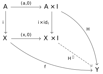
The homotopy is called the extension of with initial condition .
Definition Natural Transformation [math-000N]
Let and be categories, let be functors. A natural transformation is a function consists of
- For each , there is a morphism in , called the -component of
- For every morphism in , there is a commute diagram
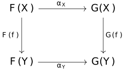
常青筆記的困難 [note-0001]
Sterling 的 https://www.forester-notes.org/QHXX/index.xml 精確的描述了常青筆記可能遭遇的困難,關鍵在於,常青筆記對於不停變化的目標,如數學、電腦程式框架等存在,本體論的目標並不統一。用數學為例,我們傳統上接受 ZFC 作為「集合論」的本體,但 topos theory 的發展給出另一套定義 ETCS https://en.wikipedia.org/wiki/Elementary_Theory_of_the_Category_of_Sets!ETCS 說我們覺得集合論是「由 sets 與 functions 構成的 well-pointed topos,有自然數 object 與 Epics split」。
這個定義並沒有循環定義(但使用了短語簡化說法),因為 sets 跟 functions 的公理可以直接給出,ETCS 並沒有比 ZFC 不穩固。
事實上我們甚至知道 ETCS 跟 ZFC 的差異,ETCS + replacement(https://en.wikipedia.org/wiki/Axiom_schema_of_replacement)等價於 ZFC 的推理能力。ZFC 中的某部份等價於 ETCS(參考 Sheaves in Geometry and Logic: A First Introduction to Topos Theory VI. 10)
重點是,既然沒辦法保證討論主題的永久不變,那就應該紀錄當下對主題的洞見,因而在未來仍可從思想中復原出結構。
Definition Pfaffian [math-000P]
Let be a skew-symmetric endomorphism of a vector space (hence can also be view as a tensor: ) and is even, the Pfaffian of is the number defined as the constant factor in the tensor equality:
where is an orthonormal basis of .
The sign of Pfaffian depends on the orientation of the orthonormal basis.
An Agda Framework for Synthetic Mathematics [math-000K]
https://samtoth.github.io/agda-synthetic-categories/index/index.xml
Theorem Borsuk–Ulam [math-000L]
If is continuous then there exists a point such that .
Lemma [math-000M]
If is continuous and antipode-preserving, then there exists a point such that .
Proof [local-0]
Use standard stereographic projection, we can see and charts gives exactly the same coordinate system at equator (i.e. where its embedding coordinate with ). This also tells the equator is a in because .
By continuous and antipode-preserving, preserves such an equator (we denote ) to (with any deformation that still an antipode shape) and must bound a set contains .
By continuous, both of two open sets of , complement of , needs to be mapped to cover the subset of which bounded by , so there exists a point such that .
Proof [local-0]
Define , is continuous.
By
is antipode-preserving.
By the lemma, there is a point such that , so then .
Determinant of Skew-Symmetric Matrices [math-000V]
This problem arose from studying the book Lectures on the Geometry of Manifolds: Suppose is a real vector space, and is a symplectic duality, then has even dimension.
I can make some concrete computation on dimension 2 and 3 and roughly understand the reason, but I have no general proof.
After a month, I found a solution:
Proof Using the properties of matrix column operations [math-000W]
Since the multiplication factor of a matrix column can be extracted as a basis, flip the column 1 (i.e. the whole column multiply ) we have
Following this pattern, flipping column 2 gives us:
Let be an skew-symmetric matrix. After flipping all columns, we obtain , therefore
By definition, skew-symmetric means , so
When is odd, this gives us
Therefore must be 0.
After formalize this statement https://github.com/dannypsnl/blackboard/commit/2c0de90a98c24ae57bd30bc47ed8c3b6a75f2664, I found this need the field is charateristic 0, sure indeed satisfies that, this point to me is that Lean can help me refine my ideas.
If represents a duality, then . Therefore cannot be odd—it must be even.
What I Wish I Knew When Learning HoTT [tt-000P]
Dependent Pattern Matching [ag-0001]
{-# OPTIONS --safe --without-K #-} module ag-0001 where open import MLTT.Spartan
依賴類型有一些不同於常見語言的特徵,像是下面定義的這個類型
data So : 𝟚 → 𝓤₀ ̇ where oh : So ₁ ho : So ₀
在模式比對時 constructor oh 跟 ho
提供了變數 b 的訊息。
xxx : {b : 𝟚} → So b → 𝟚 xxx {b} oh = b -- 這裡 b 一定是 ₁ xxx {b} ho = b -- 這裡 b 一定是 ₀
Lecture Domain Theory [dt-0000]
Programming in pcas [math-WE2N]
Categorical Realizability
Everything here works over a pca .
Definition term [local-0]
Fix a countably infinite set of variables, inductively define the set of terms over a pca :
- a variable is a term,
- an element of is a term,
- given two terms and , we may form a new term .
Definition defined terms [local-1]
A closed term is defined if, when we interpret as applied to in , all these applications are defined.
Extends to open term then is if all possible substitutions of all variables in by elements of , the obtained closed term is defined.
Definition "-abstraction" in pca [local-2]
For a variable and a term , we can define a new term by recursion on terms:
- ,
- if is a variable different from ,
- for ,
- .
Notation [local-3]
writes for
Example [local-4]
Now, we can work on it, e.g.
so
Pair and projections are
Definition The category of assemblies over a pca [math-I7R9]
Categorical Realizability
First, we define map between assemblies.
Definition assembly map [local-0]
An assembly map from an assembly to an assembly is a function that is tracked by some element.
Definition Track [math-GM4F]
For assemblies and , we say that an element tracks a function if for all and , if , then is defined and .
Then, we check assemblies and assembly maps form a category.
Proposition assemblies and assembly maps form a category [local-2]
Proof [local-1]
If and are assembly maps, then is tracked. Let and track and respectively. We claim that tracks , the closed term is defined by construction, and if then
by choice of and . Then we need identity, for each assembly , tracks any identity on , so assemblies and assembly maps form a category.
Notation [local-3]
We denote for the category of assemblies over a pca .
Example [local-4]
The trivial pca has .
Proposition terminal object [local-5]
The terminal object in is given by
Proposition products [local-6]
The product of two assemblies is given by
Proposition exponentials [local-8]
The exponential of two assemblies is given by
Proof [local-7]
The evaluation morphism is given by is tracked by . Every induces a unique assembly map making the commute diagram:
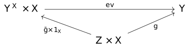
Since there is a unique assignment and the assignment is tracked by when tracks .
Proposition equalizers [local-9]
The equalizer of two assembly maps is given by
Proposition initial object [local-10]
The initial object is given by with empty realizability relation (no element so empty realizability is fine).
Proposition coproducts [local-11]
The coproduct is defined by
where
Proposition coequalizers [local-12]
The coequalizer of assembly maps is given by
where is the least equivalence relation on generated by for all .
Course CS208 Logic & Algorithms [MSP-cs208]
Code and Materials for an interactive online course on Logic (part of Strathclyde's CS208 Logic and Algorithms module)
- project link: https://github.com/msp-strath/cs208-logic
- site link: https://personal.cis.strath.ac.uk/robert.atkey/cs208/index.html
Tool agda 的開發工具 [agda-0001]
我使用的編輯器工具是 Agda Mode on VS Code,也可以用 emacs 之類的。常用操作有
ctrl+c, ctrl+l 會編譯檢查檔案,假設程式中有
?,會被替換成所謂的 hole{! !},其實就是待寫的程式ctrl+c, ctrl+, 可以窺看 hole 的目標類型,與當前 context 有哪些 term 可用
ctrl+c, ctrl+r 會把 hole 中你打的程式碼往前提取,當然前提是類型是正確的
ctrl+c, ctrl+m 會把 hole 中你打的程式碼直接當成結果,一樣類型要是正確的
一般來說一個 agda 定義如下
hello : A → B hello a = {! !}ctrl+c, ctrl+c 會問你要把哪個變數用構造子分開,回答
a,假設有a1與a2兩個構造子,程式就會變成hello : A → B hello a1 = {! !} hello a2 = {! !}
使用 Linux 的使用者可以更改預設的 copy/cut 指令以免衝突。
已完成的軟體 [software-0007]
已完成的軟體這種概念,是指一個軟體的功能已經沒有大幅度更動的必要,可以長期使用在產品上,而軟體本身只會進行必要的安全與移植性更新。我在 https://josem.co/the-beauty-of-finished-software/ 讀到這個想法。對應到筆記軟體上,我不希望軟體一直更新,尤其是當我一打開工具需要寫筆記時,上面的更新按鈕非常的讓人煩躁。同時,這個想法也是一種解放我們原先對軟體想像的開端,比起軟體如何如何,更重要的是真的去做,外部連結裡面也談到冰與火之歌正是用這樣的軟體寫出。
git send-email setup with Protonmail [software-0006]
In the original setup I already explain the configuration, to do the same with Protonmail will need to install Proton Mail Bridge(https://proton.me/mail/bridge), then with configuration as below.
[sendemail] smtpEncryption = STARTTLS smtpServer = 127.0.0.1 smtpUser = <your id>@protonmail.com smtpServerPort = 1025 smtpPass = <your password>
Definition point-surjective [math-000A]
A morphism is point-surjective iff for every point , there exists a point that lifts (satisfy ).
git send-email 的設定 [software-0004]
I use gmail, and hence, I need to get a Google app password. After having the password, one has to setup ~/.gitconfig with content:
[sendemail] smtpEncryption = tls smtpServer = smtp.gmail.com smtpUser = <your id>@gmail.com smtpServerPort = 587 smtpPass = <your password>
Then you are able to use git send-email command:
git switch -c branch-patch git format-patch main git send-email 0001-***********.patch
prompt will ask some questions, an important one is which mailing list is your target? After command success, your patch are sent.
For certain git repository you're working on, can config local repository via git config --edit, and add below to omit email list in command line.
[sendemail] to = <target email list>
Mastodon 私訊相比於一般通訊軟體 e.g. LINE, Telegram [software-0003]
好處 [local-0]
- 可以有效分類特定話題,例如一個串是講約去哪裡吃飯、另一個串講專業內容
- 可以用僅限提及的人,限制可見性,所以可以形成一定程度的群組概念
壞處 [local-1]
- 兩方站點的站長都能看到內容
- 客戶端不支援把一群提及名單固定成群組,這或許是一個可行的客戶端新功能
壞處的可能解法:公佈自己的 public key 讓對方加密訊息再傳,配上專用客戶軟體或許可以做的更方便
let Racket GC manage your FFI object [software-0005]
All you need are deallocator and allocator from ffi/unsafe/alloc.
(require ffi/unsafe
ffi/unsafe/define
ffi/unsafe/alloc)
(define-ffi-definer define-xxx
(ffi-lib "" '(#f)))
(define-xxx free-yyy (_fun _YyyRef -> _void)
#:c-id yyy_delete
#:wrap (deallocator))
(define-xxx make-yyy (_fun -> _YyyRef)
#:c-id yyy_new
#:wrap (allocator free-yyy)) Tool ngrok [software-0002]
Sometimes we didn't have public ip, but temporary wants to test website, ngrok can help in this situation.
# expose localhost:8080 by HTTP $ ngrok http 8080 # expose localhost:8080 by TCP $ ngrok tcp 8080
XDP [software-0001]
XDP is eXpress Data Path, it's a technology about putting a BPF code virtual machine on the NIC(network interface controller) driver before kernel network stack so that we can filter the packet before kernel, it would make processing speed greater.
We can do following things on the packet:
XDP_PASS: allow the packet to pass throughXDP_DROP: drop the packetXDP_TX: bounce the packet back on the same interfaceXDP_REDIRECT: redirects the packet to another interface
Here is an example of counting how many IPv4/6 packets be dropped.
package main
import (
"fmt"
"os"
"os/signal"
bpf "github.com/iovisor/gobpf/bcc"
)
// bcc is from iovisor/bcc this project
/*
#cgo CFLAGS: -I/usr/include/bcc/compat
#cgo LDFLAGS: -lbcc
#include
#include
void perf_reader_free(void *ptr);
*/
import "C"
const source string = `
#define KBUILD_MODNAME "foo"
#include
#include
#include
#include
#include
#include
#include
BPF_TABLE("array", int, long, dropcnt, 256);
static inline int parse_ipv4(void *data, u64 nh_off, void *data_end) {
struct iphdr *iph = data + nh_off;
if ((void*)&iph[1] > data_end)
return 0;
return iph->protocol;
}
static inline int parse_ipv6(void *data, u64 nh_off, void *data_end) {
struct ipv6hdr *ip6h = data + nh_off;
if ((void*)&ip6h[1] > data_end)
return 0;
return ip6h->nexthdr;
}
int xdp_prog1(struct xdp_md *ctx) {
void* data_end = (void*)(long)ctx->data_end;
void* data = (void*)(long)ctx->data;
struct ethhdr *eth = data;
uint64_t nh_off = sizeof(*eth);
if (data + nh_off > data_end)
return XDP_DROP;
uint16_t h_proto = eth->h_proto;
if (h_proto == htons(ETH_P_8021Q) || h_proto == htons(ETH_P_8021AD)) {
struct vlan_hdr *vhdr;
vhdr = data + nh_off;
nh_off += sizeof(struct vlan_hdr);
if (data + nh_off > data_end)
return XDP_DROP;
h_proto = vhdr->h_vlan_encapsulated_proto;
}
if (h_proto == htons(ETH_P_8021Q) || h_proto == htons(ETH_P_8021AD)) {
struct vlan_hdr *vhdr;
vhdr = data + nh_off;
nh_off += sizeof(struct vlan_hdr);
if (data + nh_off > data_end)
return XDP_DROP;
h_proto = vhdr->h_vlan_encapsulated_proto;
}
int index;
if (h_proto == htons(ETH_P_IP))
index = parse_ipv4(data, nh_off, data_end);
else if (h_proto == htons(ETH_P_IPV6))
index = parse_ipv6(data, nh_off, data_end);
else
index = 0;
long *value;
value = dropcnt.lookup(&index);
if (value) lock_xadd(value, 1);
return XDP_DROP;
}
`
func usage() {
fmt.Printf("Usage: %v \n", os.Args[0])
fmt.Printf("e.g.: %v eth0\n", os.Args[0])
os.Exit(1)
}
func main() {
if len(os.Args) != 2 {
usage()
}
module := bpf.NewModule(source, []string{
"-w",
})
defer module.Close()
fn, err := module.Load("xdp_prog1", C.BPF_PROG_TYPE_XDP, 1, 65536)
if err != nil {
fmt.Fprintf(os.Stderr, "Failed to load xdp prog: %v\n", err)
os.Exit(1)
}
device := os.Args[1]
if err := module.AttachXDP(device, fn); err != nil {
fmt.Fprintf(os.Stderr, "Failed to attach xdp prog: %v\n", err)
os.Exit(1)
}
defer func() {
if err := module.RemoveXDP(device); err != nil {
fmt.Fprintf(os.Stderr, "Failed to remove XDP from %s: %v\n", device, err)
}
}()
fmt.Println("Dropping packets, hit CTRL+C to stop")
sig := make(chan os.Signal, 1)
signal.Notify(sig, os.Interrupt, os.Kill)
dropcnt := bpf.NewTable(module.TableId("dropcnt"), module)
<-sig
fmt.Println("\n{IP protocol-number}: {total dropped pkts}")
for it := dropcnt.Iter(); it.Next(); {
key := bpf.GetHostByteOrder().Uint32(it.Key())
value := bpf.GetHostByteOrder().Uint64(it.Leaf())
if value > 0 {
fmt.Printf("%v: %v pkts\n", key, value)
}
}
} Algorithm Mark sweep GC [cs-0008]
Mark-Sweep is a classic GC algorithm, it's combined with two parts, mark and sweep.
mark(root):
if not marked?(root):
mark(root)
for obj in knowns(root):
mark(obj)
sweep(heap):
for obj in heap:
if marked?(obj):
unmark(obj)
else:
release(obj)
If we run collection (mark-sweep), then since each object is reachable from root, so no one would be released.
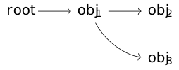
After do some executions, obj1 don't need obj3 anymore, so it became:
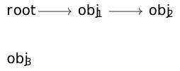
Now when we run collection, obj3 is unreachable from root, so it won't be marked! When running to sweep, it will be dropped.